Point-Curve Constraint (SimMechanics)

Constrain the motion of a point on one body to be along a curve on another body

Library

Constraints & Drivers

Description

The two Bodies connected by a Point-Curve Constraint can only move relative to one another if a point on one body moves along a curve on the other body. The point on one body is the origin of the Body coordinate systems (CS) to which one side of the Point-Curve Constraint is connected. The corresponding curve starting point on the other body is the origin of the Body CS to which the other side of the Point-Curve Constraint is connected.

Specifying the Curve You specify the curve function on the second body as a spline with break points and end conditions. The spline is a piecewise cubic polynomial, with the pieces joined at user-specified breakpoints:

₁

) , (x

₂

) , ... , (x

)

and boundary conditions applied at the spline's endpoints, (x₀,y₀,z₀) and (x_N+1,y_N+1,z_N+1). The spline curve and its first two derivatives are continuous at each breakpoint.

Constraints restrict relative degrees of freedom (DoFs) between a pair of bodies. Locally in a machine, they replace a Joint as the expression of the DoFs. Globally, Constraint blocks must occur topologically in closed loops. Like Bodies connected to a Joint, the two Bodies connected to a Constraint are ordered as base and follower, fixing the direction of relative motion.

For the Point-Curve Constraint, the base is the Body carrying the Point, and the follower is the Body carrying the Curve. The Point-Curve Constraint is assembled: the Body CS origin on the base (Point) body must initially be collocated with the Body CS origin on the follower (Curve) body, to within assembly tolerance.

You can connect a Constraint block to a Constraint & Driver Sensor, but not to an Actuator. The Constraint & Driver Sensor measures the reaction forces/torques between the constrained bodies.

Dialog Box and Parameters

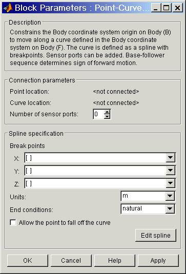
The dialog box has two active areas, Connection parameters and Spline specification. It stores the defining information of a single spline for the constraint.

Connection Parameters

Current base: When you connect the base (B) Connector Port on the Point-Curve Constraint block to a Body CS Port on a Body, this parameter is automatically reset to the name of this Body CS. See the following Point-Curve Constraint base and follower Body Connector Ports figure.; This Body CS origin is the point of the Point-Curve Constraint.
Current follower: When you connect the follower (F) Connector Port on the Point-Curve Constraint block to a Body CS Port on a Body, this parameter is automatically reset to the name of this Body CS. See the following Point-Curve Constraint base and follower Body Connector Ports figure.; This Body CS origin is the starting point of the curve of the Point-Curve Constraint.
Number of sensor ports: Using this spinner menu, you can set the number of extra Connector Ports needed for connecting Constraint & Driver Sensor blocks to this Constraint. The default is 0.

The base (B)-follower (F) Body sequence determines the sense of positive motion. Positive translation is the follower moving in the direction of the translation axis.

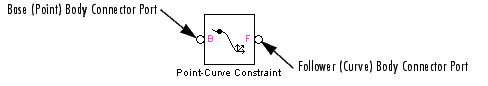
Point-Curve Constraint base and follower Body Connector Ports

Spline Specification

The Point-Curve Constraint dialog box gives you two ways to specify the spline curve. The first way is entering in this dialog box the coordinates of breakpoints and endpoints on the follower and is valid for defining curves in up to three dimensions.

The second way is graphically displaying and editing the spline in the Edit spline editor (see following), valid only for two-dimensional curves on the follower.

Break points

List here the x-components, the y-components, and the z-components, respectively, of the breakpoints and endpoints that define the spline:

X: enter (x₀, x₁, ..., x_N+1) as a vector.

Y: enter (y₀, y₁, ..., y_N+1) as a vector.

Z: enter (z₀, z₁, ..., z_N+1) as a vector.

All three fields require nonnull entries. The number of components in each vector should be the same. Exception and shortcut: if all the Z components are the same, just enter one number in the Z vector. The Break points list replicates this number to expand out a full vector.

If there are no X and/or Y components, you must still enter [0 ... 0] in that/those field(s). If there are no Z components, you must still enter at least [0] in the Z field (using the replication/expansion shortcut).

The pull-down menu for each spatial dimension lists the history of those previous breakpoints created by the graphical spline editor (see following) within a single dialog box session. Closing the dialog box destroys this history, and only the current breakpoint list is retained.

Units

In the pull-down menu, choose the linear units for distances on the constrained bodies. The default is m (meters).

End conditions

In the pull-down menu, choose the type of end (boundary) condition on the spline curve. The possible conditions are:


End Condition	Definition	Minimum Number of Points
`natural`	Match each endslope to the slope of the cubic that fits the first four points at that end	Two points
`not-a-knot`	Only the curve and its first derivative are continuous at first and last interior points	Four points
`periodic`	Match the first and second derivatives of the two endpoints	Two points, three recommended

The default is natural. The periodic end condition closes the spline.

Allow the point to fall off the curve

If the check box is selected, the base point continues with unconstrained motion if it reaches an endpoint and leaves the spline on the follower. The direction of motion at the instant the base point leaves the constraint is tangent to the spline.

If the check box is unselected, and the base point attempts to leave the spline on the follower, the simulation stops with an error. The default is unselected.

Edit spline

Click here to open the optional Edit spline dialog box.

The Edit spline dialog box provides alternative numerical entry and graphical editing methods for defining the constraint spline. But it can define only two-dimensional curves in the x-y coordinate directions on the follower Body. The Edit spline editor ignores any z-components in existing breakpoints.

Edit Spline

The numerical entry area lies on the left side of the Edit spline dialog box, the graphical editing area on the right side.

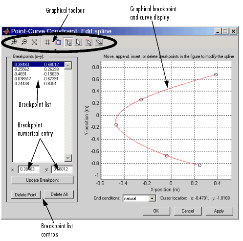
Point-Curve Constraint Spline Editor

Graphical Editing of Spline Points

To place a breakpoint in the graphical display, place your cursor at the position where you want the breakpoint. The Cursor location display in the lower right indicates your current cursor coordinates in the display.
Then click at the desired point. A circle appears where you clicked, and simultaneously, the breakpoint is listed in the Breakpoints (x-y) list.

Continuing to add breakpoints generates the spline (red curve).

Use the Graphical toolbar controls to edit the spline graphically in the display:

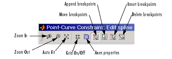
Remove points by clicking on the Delete breakpoints icon. Your cursor turns into an eraser symbol. With it, select and click the breakpoints you want to delete.
Insert new (interior) breakpoints by clicking on the Insert breakpoints icon. Your cursor acquires a small circle. Click on the positions, near the existing curve, where you want the new breakpoints. The editor modifies the spline to fit the new breakpoints.
Add new endpoints and extend the curve by clicking on the Append breakpoints icon. Your cursor acquires a small circle. Click on the positions, near the existing endpoints, to where you want to extend the curve. The editor modifies the spline to fit the new endpoints.
Move existing endpoints by clicking on the Move breakpoints icon. Click and drag the breakpoints you want to move, then drop them where you want them.

The editor modifies both the spline red curve in the graphical display and the Breakpoints (x-y) list as you make these changes.

Additional graphical toolbar controls:

Zoom In/Zoom Out and Auto Fit: Standard Handle Graphics zooming and auto resizing of graphics display.
Grid On/Off: Turn the graphical display x-y grid on or off.
Axes properties: Edit properties of graphical display.

Numerical Editing of Spline Points

Use the numerical entry controls, instead of the graphical editing tools, to edit breakpoints by text entry.

Breakpoints (x-y): You can also add, delete, and edit the breakpoints via this Breakpoints list:; Select an existing breakpoint by highlighting it with your cursor.; Add a breakpoint by moving the highlighted selection to the empty line below the last breakpoint with your cursor control.; In x: and y: enter the x- and y-coordinates of the currently selected breakpoint.
Update breakpoint: After editing an existing breakpoint or entering a new one, update the breakpoint list by clicking here. The new or changed breakpoint appears in the graphical display as a circle.
Delete point: Click here to delete the currently selected breakpoint.
Delete all: Click here to delete all the breakpoints in the Breakpoint list.
End conditions: In the pull-down menu, choose the type of end (boundary) condition on the spline curve. The possible conditions are natural, not-a-knot, and periodic. The default is natural.

Closing the Edit spline dialog box

Clicking on Apply or OK updates the breakpoints stored in the main Point-Curve Constraint dialog box.

Previous breakpoint lists are stored in the history pull-down menus of the main Point-Curve Constraint dialog box's Break points list. This history is destroyed if you close the main dialog box, and only the current Breakpoint list is retained.

See Also

Constraint & Driver Sensor

See Modeling Constraints and Drivers for more on restricting DoFs with Constraints.

See Checking Schematic Topology and How SimMechanics Works for more on using constraints in closed loops.

See Creating Constraints and Drivers.

For more about representing curves as splines, see the Spline Toolbox User's Guide tutorial.

Planar Prismatic