Tutorial (GARCH Toolbox)

GARCH Toolbox

Pre-Estimation Analysis

The pre-estimation analysis:

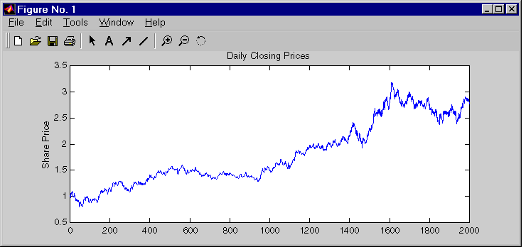
Load the Raw Data: Daily Closing Prices

Start by loading the MATLAB binary file xyz.mat, and examining its contents using the whos command.

load xyz
whos
  Name         Size         Bytes  Class

  prices    2001x1          16008  double array

Grand total is 2001 elements using 16008 bytes

The whos command lists all the variables in the current workspace, together with information about their size, bytes, and class.

The data you loaded from xyz.mat consists of a single column vector, prices, of length 2001. This vector contains the daily closing prices of the XYZ Corporation. Use the MATLAB plot function to examine the data (see plot in the online MATLAB Function Reference).

plot([0:2000], prices)
ylabel('Share Price')
title('Daily Closing Prices')

Figure 2-5: Daily Closing Prices of the XYZ Corporation

The plot shown in Figure 2-5, Daily Closing Prices of the XYZ Corporation is the same as the one shown in Figure 2-3, Typical Equity Price Series.

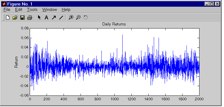
Convert the Prices to a Return Series

Because GARCH modeling assumes a return series, you need to convert the prices to returns. Use the utility function price2ret, and then examine the result.

xyz = price2ret(prices);
whos
  Name         Size         Bytes  Class

  prices    2001x1          16008  double array
  xyz       2000x1          16000  double array

Grand total is 4001 elements using 32008 bytes

The workspace information shows both the 2001-point price series and the 2000-point return series derived from it.

Now, use the MATLAB plot function to see the return series.

plot(xyz)
ylabel('Return')
title('Daily Returns')

Figure 2-6: Raw Return Series Based on Daily Closing Prices

The results, shown in Figure 2-6, Raw Return Series Based on Daily Closing Prices, are the same as those shown in Figure 2-4, Continuously Compounded Returns Associated with the Price Series. Notice the presence of volatility clustering in the raw return series.

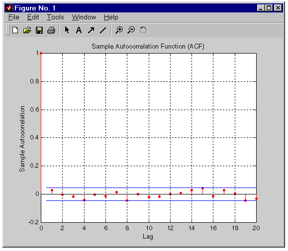
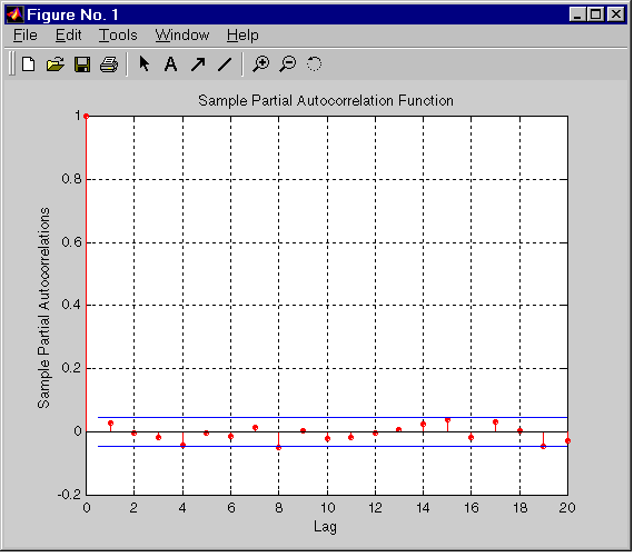
Check for Correlation

In the Return Series. You can check qualitatively for correlation in the raw return series by calling the functions autocorr and parcorr to examine the sample autocorrelation function (ACF) and partial-autocorrelation (PACF) function, respectively.

```
autocorr(xyz)
```

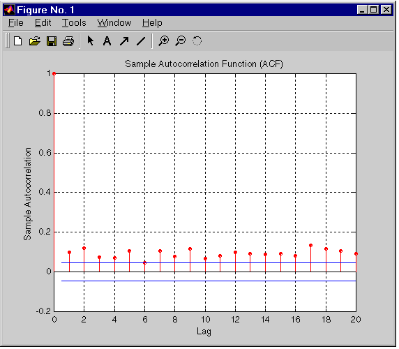
Figure 2-7: ACF with Bounds for the Raw Return Series

The autocorr function computes and displays the sample ACF of the returns, along with the upper and lower standard deviation confidence bounds, based on the assumption that all autocorrelations are zero beyond lag zero.

```
parcorr(xyz)
```

Figure 2-8: PACF with Bounds for the Raw Return Series

Similarly, the parcorr function displays the sample PACF with upper and lower confidence bounds.

Since the individual ACF values can have large variances and can also be autocorrelated, you should view the sample ACF and PACF with care (see Box, Jenkins, Reinsel [7], pages 34 and 186). However, as preliminary identification tools, the ACF and PACF provide some indication of the broad correlation characteristics of the returns. From Figure 2-7, ACF with Bounds for the Raw Return Series and Figure 2-8, PACF with Bounds for the Raw Return Series, there is no real indication that you need to use any correlation structure in the conditional mean. Also, notice the similarity between the graphs.

In the Squared Returns. Although the ACF of the observed returns exhibits little correlation, the ACF of the squared returns may still indicate significant correlation and persistence in the second-order moments. Check this by plotting the ACF of the squared returns.

```
autocorr(xyz.^2)
```

Figure 2-9: ACF of the Squared Returns

Figure 2-9, ACF of the Squared Returns shows that, although the returns themselves are largely uncorrelated, the variance process exhibits some correlation. This is consistent with the earlier discussion in the section, The Default Model. Note that the ACF shown in Figure 2-9, ACF of the Squared Returns appears to die out slowly, indicating the possibility of a variance process close to being nonstationary.

Note The syntax in the preceding command, an operator preceded by the dot operator (.), indicates that the operation is performed on an element-by-element basis. In the preceding command, xyz.^2 indicates that each element of the vector xyz is squared.

Quantify the Correlation

You can quantify the preceding qualitative checks for correlation using formal hypothesis tests, such as the Ljung-Box-Pierce Q-test and Engle's ARCH test.

The function lbqtest implements the Ljung-Box-Pierce Q-test for a departure from randomness based on the ACF of the data. The Q-test is most often used as a post-estimation lack-of-fit test applied to the fitted innovations (i.e., residuals). In this case, however, you can also use it as part of the pre-fit analysis because the default model assumes that returns are just a simple constant plus a pure innovations process. Under the null hypothesis of no serial correlation, the Q-test statistic is asymptotically Chi-Square distributed (see Box, Jenkins, Reinsel [7], page 314).

The function archtest implements Engle's test for the presence of ARCH effects. Under the null hypothesis that a time series is a random sequence of Gaussian disturbances (i.e., no ARCH effects exist), this test statistic is also asymptotically Chi-Square distributed (see Engle [8], pages 999-1000).

Both functions return identical outputs. The first output, H, is a Boolean decision flag. H = 0 implies that no significant correlation exists (i.e., do not reject the null hypothesis). H = 1 means that significant correlation exists (i.e., reject the null hypothesis). The remaining outputs are the P-value (pValue), the test statistic (Stat), and the critical value of the Chi-Square distribution (CriticalValue).

Ljung-Box-Pierce Q-Test. Using lbqtest, you can verify, at least approximately, that no significant correlation is present in the raw returns when tested for up to 10, 15, and 20 lags of the ACF at the 0.05 level of significance.

[H, pValue, Stat, CriticalValue] = lbqtest(xyz-mean(xyz), [10 15 
20]', 0.05);
[H  pValue  Stat  CriticalValue]
ans =
         0    0.2996   11.7869   18.3070
         0    0.2791   17.6943   24.9958
         0    0.1808   25.5616   31.4104

However, there is significant serial correlation in the squared returns when you test them with the same inputs.

[H, pValue, Stat, CriticalValue] = lbqtest((xyz-mean(xyz)).^2, 
[10 15 20]', 0.05);
[H  pValue  Stat  CriticalValue]
ans =
    1.0000         0  177.5937   18.3070
    1.0000         0  263.9325   24.9958
    1.0000         0  385.6907   31.4104

Engle's ARCH Test. You can also perform Engle's ARCH test using the function archtest. This test also shows significant evidence in support of GARCH effects (i.e heteroscedasticity).

[H, pValue, Stat, CriticalValue] = archtest(xyz-mean(xyz), [10 15 
20]', 0.05);
[H  pValue  Stat  CriticalValue]
ans =
    1.0000         0  107.6171   18.3070
    1.0000         0  127.1083   24.9958
    1.0000         0  159.6543   31.4104

Each of these examples extracts the sample mean from the actual returns. This is consistent with the definition of the conditional mean equation of the default model, in which the innovations process is _t = y_t - C, and C is the mean of y_t.

Analysis and Estimation Example Using the Default Model Parameter Estimation