| DSP Blockset | |
Solve a linear system of equations using Levinson-Durbin recursion.
Library
Math Functions / Matrices and Linear Algebra / Linear System Solvers
Description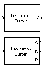
The Levinson-Durbin block solves the nth-order system of linear equations

for the particular case where R is a Hermitian, positive-definite, Toeplitz matrix and b is identical to the first column of R shifted by one element and with the opposite sign.
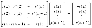
The input to the block, r = [r(1) r(2) ... r(n+1)], can be a 1-D or 2-D vector (row or column). It contains lags 0 through n of an autocorrelation sequence, which appear in the matrix R.
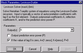
The block can output the polynomial coefficients, A, the reflection coefficients, K, and the prediction error power, P, in various combinations. The Output(s) parameter allows you to enable the A and K outputs by selecting one of the following settings:
A outputs A=[1 a(2) a(3) ... a(n+1)], the solution to the Levinson-Durbin equation. A has the same dimension as the input. The elements of the output can also be viewed as the coefficients of an nth-order autoregressive (AR) process (see below).
K outputs K=[k(1) k(2) ... k(n)], which contains n reflection coefficients, and has the same dimension as the input, less one element. (A scalar input causes an error when K is selected.) Reflection coefficients are useful for realizing a lattice representation of the AR process described below.
Both A and K are always 1-D vectors.
The prediction error power, P, (a scalar), is output when the Output prediction error power (P) check box is selected. P represents the power of the output of an FIR filter with taps A and input autocorrelation described by r, where A represents a prediction error filter and r is the input to the block. (In this case, A is a whitening filter).
When If the value of lag 0 is zero, A=[1 zeros], K=[zeros], P=0 is selected (default), an input whose r(1) element is zero generates a zero-valued output. When this check box is not selected, an input with r(1) = 0 generates NaNs in the output. In general, an input with r(1) = 0 is invalid because it does not construct a positive-definite matrix R; however, it is common for blocks to receive zero-valued inputs at the start of a simulation. The check box allows you to avoid propagating NaNs during this period.
Applications
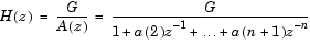
One application of the Levinson-Durbin formulation above is in the Yule-Walker AR problem, which concerns modeling an unknown system as an autoregressive process. Such a process would be modeled as the output of an all-pole IIR filter with white Gaussian noise input. In the Yule-Walker problem, the use of the signal's autocorrelation sequence to obtain an optimal estimate leads to an Ra = b equation of the type shown above, which is most efficiently solved by Levinson-Durbin recursion. In this case, the input to the block represents the autocorrelation sequence, with r(1) being the zero-lag value. The output at the block's A port then contains the coefficients of the autoregressive process that optimally models the system. The coefficients are ordered in descending powers of z, and the AR process is minimum phase. The prediction error, G, defines the gain for the unknown system, where  .
.
The output at the block's K port contains the corresponding reflection coefficients, [k(1) k(2) ... k(n)], for the lattice realization of this IIR filter. The Yule-Walker AR Estimator block implements this autocorrelation-based method for AR model estimation, while the Yule-Walker Method block extends the method to spectral estimation.
Another common application of the Levinson-Durbin algorithm is in linear predictive coding, which is concerned with finding the coefficients of a moving average (MA) process (or FIR filter) that predicts the next value of a signal from the current signal sample and a finite number of past samples. In this case, the input to the block represents the signal's autocorrelation sequence, with r(1) being the zero-lag value, and the output at the block's A port contains the coefficients of the predictive MA process (in descending powers of z).

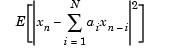
These coefficients solve the optimization problem below.

Again, the output at the block's K port contains the corresponding reflection coefficients, [k(1) k(2) ... k(n)], for the lattice realization of this FIR filter. The Autocorrelation LPC block in the Linear Prediction library implements this autocorrelation-based prediction method.
Algorithm
The algorithm requires O(n2) operations, and is thus much more efficient for large n than standard Gaussian elimination, which requires O(n3) operations.
Dialog Box
P.r(1) = 0. When cleared, the block outputs NaNs for these inputs.References
Golub, G. H., and C. F. Van Loan. Sect. 4.7 in Matrix Computations. 3rd ed. Baltimore, MD: Johns Hopkins University Press, 1996.
Ljung, L. System Identification: Theory for the User. Englewood Cliffs, NJ: Prentice Hall, 1987. Pgs. 278-280.
Kay, Steven M., Modern Spectral Estimation: Theory and Application. Englewood Cliffs, NJ: Prentice Hall, 1988.
Supported Data Types
To learn how to convert to the above data types in MATLAB and Simulink, see Supported Data Types and How to Convert to Them.
See Also
| Cholesky Solver |
DSP Blockset |
| LDL Solver |
DSP Blockset |
| Autocorrelation LPC |
DSP Blockset |
| LU Solver |
DSP Blockset |
| QR Solver |
DSP Blockset |
| Yule-Walker AR Estimator |
DSP Blockset |
| Yule-Walker Method |
DSP Blockset |
levinson |
Signal Processing Toolbox |
See Solving Linear Systems for related information. Also see Linear System Solvers for a list of all the blocks in the Linear System Solvers library.
| | Least Squares Polynomial Fit | LMS Adaptive Filter | |