DSP Blockset

Autocorrelation LPC

Determine the coefficients of an Nth-order forward linear predictor.

Library

Estimation / Linear Prediction

Description

The Autocorrelation LPC block determines the coefficients of an N-step forward linear predictor for the time-series in length-M input vector, u, by minimizing the prediction error in the least-squares sense. A linear predictor is an FIR filter that predicts the next value in a sequence from the present and past inputs. This technique has applications in filter design, speech coding, spectral analysis, and system identification.

The Autocorrelation LPC block can output the prediction error as polynomial coefficients, reflection coefficients, or both. It can also output the prediction error power. The length-M input, u, can be a scalar, 1-D vector, frame- or sample-based column vector, or a sample-based row vector. Frame-based row vectors are not valid inputs.

When Inherit prediction order from input dimensions is selected, the prediction order, N, is inherited from the input dimensions. Otherwise, the Prediction order parameter sets the value of N.

When Output(s) is set to A, port A is enabled. Port A outputs an (N+1)-by-1 column vector, a = [1 a₂ a₃ ... a_N+1]^T, containing the coefficients of an Nth-order moving average (MA) linear process that predicts the next value, û_M+1, in the input time-series.

When Output(s) is set to K, port K is enabled. Port K outputs a length-N column vector whose elements are the prediction error reflection coefficients. When Output(s) is set to A and K, both port A and K are enabled, and each port outputs its respective column vector of prediction coefficients. The outputs at both port A and K are always 1-D vectors.

When Output prediction error power (P) is selected, port P is enabled. The prediction error power, a scalar, is output at port P.

Algorithm

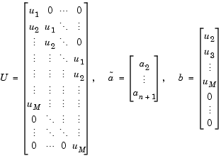
The Autocorrelation LPC block computes the least-squares solution to

where indicates the 2-norm and

Solving the least-squares problem via the normal equations

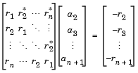
leads to the system of equations

where r = [r₁ r₂ r₃ ... r_n+1]^T is an autocorrelation estimate for u computed using the Autocorrelation block, and * indicates the complex conjugate transpose. The normal equations are solved in O(n²) operations by the Levinson-Durbin block.

Note that the solution to the LPC problem is very closely related to the Yule-Walker AR method of spectral estimation. In that context, the normal equations above are referred to as the Yule-Walker AR equations.

Dialog Box

Output(s)

The type of prediction coefficients output by the block. The block can output polynomial coefficients (A), reflection coefficients (K), or both (A and K).

Output prediction error power (P)

When selected, enables port P, which outputs the output prediction error power.

Inherit prediction order from input dimensions

When selected, the block inherits the prediction order from the input dimensions.

Prediction order (N)

The prediction order, N. This parameter is disabled when Inherit prediction order from input dimensions is selected.

References

Haykin, S. Adaptive Filter Theory. 3rd ed. Englewood Cliffs, NJ: Prentice Hall, 1996.

Ljung, L. System Identification: Theory for the User. Englewood Cliffs, NJ: Prentice Hall, 1987. Pgs. 278-280.

Proakis, J. and D. Manolakis. Digital Signal Processing. 3rd ed. Englewood Cliffs, NJ: Prentice-Hall, 1996.

Supported Data Types

• Double-precision floating point
• Single-precision floating point

To learn how to convert to the above data types in MATLAB and Simulink, see Supported Data Types and How to Convert to Them.

See Also

Autocorrelation	DSP Blockset
Levinson-Durbin	DSP Blockset
Yule-Walker Method	DSP Blockset
lpc	Signal Processing Toolbox

Also see Linear Prediction for a list of all the blocks in the Linear Prediction library.

Autocorrelation

Backward Substitution