splinetool (Spline Toolbox)

Experiment with some spline approximation methods

Syntax

```
splinetool
splinetool(x,y) 
```

Description

splinetool is a graphical user interface (GUI), whose initial menu provides you with various choices for data including the option of importing some data from the workspace.

splinetool(x,y) brings up the GUI with the specified data x and y, which are vectors of the same length.

Remarks

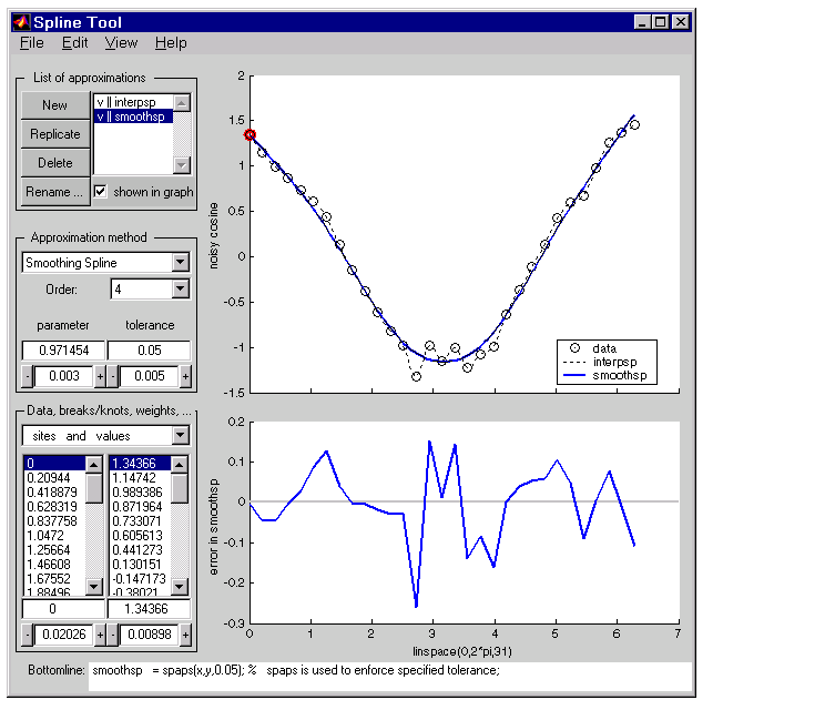
The Spline Tool is shown below comparing cubic spline interpolation with a smoothing spline on sample data created by adding noise to the cosine function.

Approximation Methods

The approximation methods and options supported by the GUI are shown below.

Approximation Method
Option

Cubic Interpolating Spline
Adjust the type and values of the end conditions.

Smoothing Spline
Choose between cubic (order 4) and quintic (order 6) splines. Adjust the value of the tolerance and/or smoothing parameter. Adjust the weights in the error and roughness measures.

Least-Squares Approximation
Vary the order from 1 to 14. The default order is 4, which gives cubic approximating splines. Modify the number of polynomial pieces. Add and move knots to improve the fit. Adjust the weights in the error measure.

Spline Interpolation
Vary the order from 2 to 14. The default order is 4, which gives cubic spline interpolants. If the default knots supplied are not satisfactory, you can move them around to vary the fit.

Approximation Method	Option
Cubic Interpolating Spline	Adjust the type and values of the end conditions.
Smoothing Spline	Choose between cubic (order 4) and quintic (order 6) splines. Adjust the value of the tolerance and/or smoothing parameter. Adjust the weights in the error and roughness measures.
Least-Squares Approximation	Vary the order from 1 to 14. The default order is 4, which gives cubic approximating splines. Modify the number of polynomial pieces. Add and move knots to improve the fit. Adjust the weights in the error measure.
Spline Interpolation	Vary the order from 2 to 14. The default order is 4, which gives cubic spline interpolants. If the default knots supplied are not satisfactory, you can move them around to vary the fit.

Graphs

You can generate and compare several approximations to the same data. One of the approximations is always marked as "current" using a thicker line width. The following displays are available:

Data graph. It shows:

The data
The approximations chosen for display in List of approximations
The current knot sequence or the current break sequence

Auxiliary graph (if viewed) for the current approximation. You can invoke this graph by selecting any one of the items in the View menu. It shows one of the following:

The first derivative
The second derivative
The error

By default, the error is the difference between the given data values and the value of the approximation at the data sites. In particular, the error is zero (up to round-off) when the approximation is an interpolant. However, if you provide the data values by specifying a function, then the error displayed is the difference between that function and the current approximation. This also happens if you change the y-label of the data graph to the name of a function.

Menu Options

You can annotate and print the graphs with the File -> Print Graph menu.

You can export the data and approximations to the workspace for further use or analysis with the File -> Export Data and File -> Export Spline menus, respectively.

You can create, with the File -> Save M-file menu, a function M-file that you can use to generate, from the original data, any or all graphs currently shown. This M-file also provides you with a written record of the spline toolbox commands used to generate the current graph(s).

You can save, with the Replicate button, the current approximation before you experiment further. If, at a later time, you click on the approximation so saved, splinetool restores everything to the way it was, including the data used in the construction of the saved approximation. This is true even if, since saving this approximation, you have edited the data while working on other approximations.

You can add, delete, or move data, knots, and breaks by right-clicking in the graph, or selecting the appropriate item in the Edit menu.

Examples

Exploring End Conditions For Cubic Spline Interpolation

The purpose of this example is to explore the various end conditions available with cubic spline interpolation:

Type splinetool at the command line.
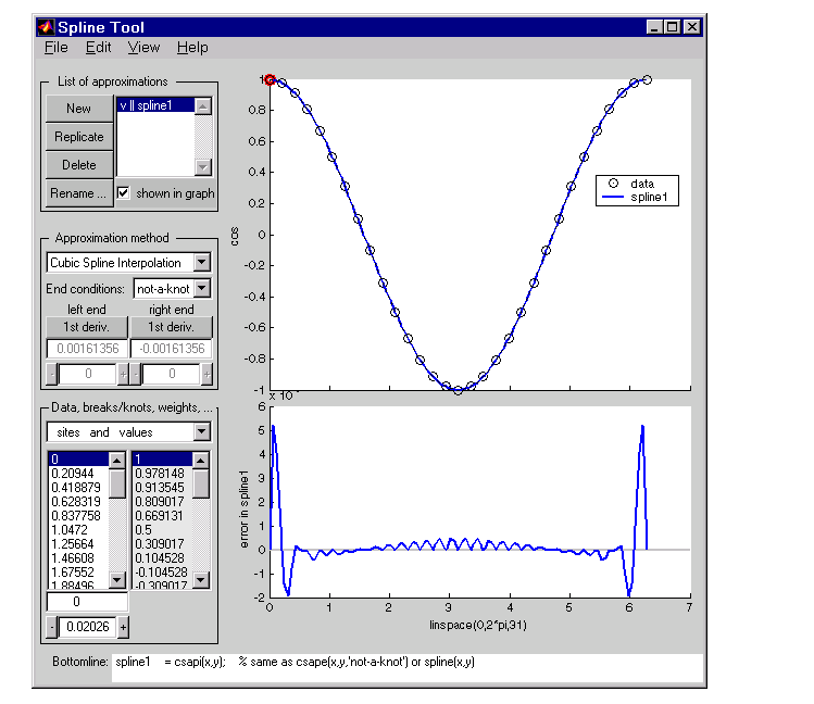
Select Provide your own data from the initial screen, and accept the default function. You should see the following display.

The default approximation shown is the cubic spline interpolant with the not-a-knot end condition.

The vector x of data sites is linspace(0,2*pi,21) and the values given by cos(x). This differs from simply providing the vector y of values in that the cosine function is explicitly recorded as the underlying function. Therefore, the error shown in the graph is the error in the spline as an approximation to the cosine rather than as an approximation to the given values. Notice the resulting relatively large error, about 5e-5, near the endpoints.

For comparison, follow these steps:

Click on New in the List of approximations.
In Approximation method, select complete from the list of End conditions.
Since the first derivative of the cosine function is sine, adjust the first-derivative values to their known values of zero at both the left end and the right end.

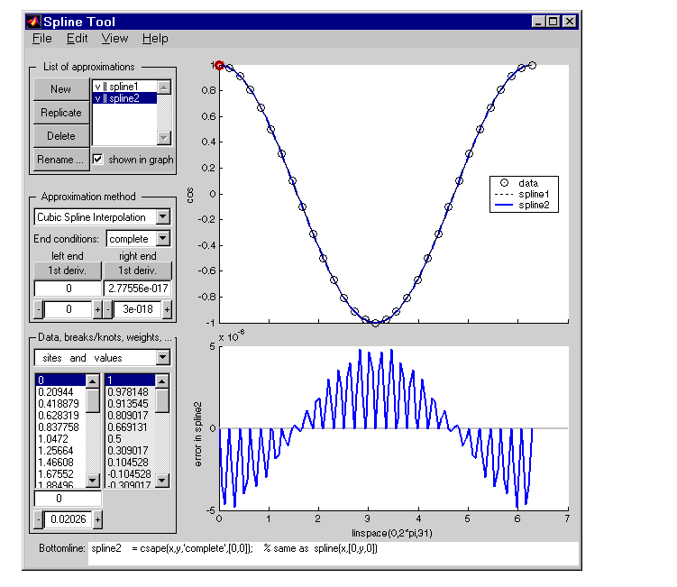
This procedure results in the display shown below. Note that the right end slope is zero only up to round-off. Bottomline tells you that the toolbox function csape was used to create the spline.

Be impressed by the improvement in the error, which is only about 5e-6.

For further comparison, follow these steps:

Click on New in the List of approximations.
In Approximation method, select 'natural' from the list of End conditions.

Note the deterioration of the approximation near the ends, an error of about 2e-3, which is much worse than with the not-a-knot end conditions.

For a final comparison, follow these steps:

Click on New in the List of approximations.
Since we know that the cosine function is periodic, in Approximation method, select periodic from the list of End conditions.

Note the dramatic improvement in the approximation, back to an error of about 5e-6, particularly compared to the 'natural' end conditions.

Estimating the Second Derivative at an Endpoint

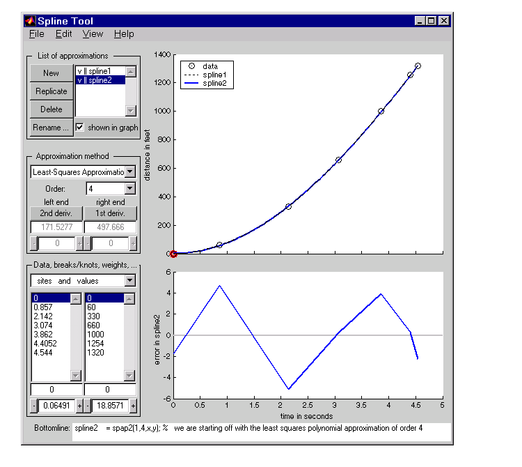
This example uses cubic spline interpolation and least-squares approximation to determine an estimate of the initial acceleration for a drag car:

Type splinetool at the command line or if the GUI is already running, click on File->Restart.
Choose Richard Tapia's drag racing data. These data show the distance traveled by a drag car as a function of time.
In Approximation method, select complete from the list of End conditions.
Adjust the initial speed by changing the first derivative at the left endpoint to zero.
Look for the value of the initial acceleration, which is given by the value of the second derivative at the left endpoint. You can toggle between the first derivative and the second derivative at this endpoint by clicking on the left end button. The value of the second derivative should be around 187 in the units chosen. Choose View->Show 2nd Derivative to see this graphically.
For comparison, click on New, then choose Least-Squares Approximation as the Approximation method. With this method, you can no longer specify end conditions. Instead, you may vary the order of the method. Verify that the initial acceleration is close to the cubic interpolation value.

The results of this procedure are shown below.

Least-Squares Approximation

This example encourages you to place five interior knots in such a way that the least-squares approximation to these data by cubic splines has an absolute error no bigger than .04 everywhere:

Type splinetool at the command line or if the GUI is already running, click on File->Restart.
Choose Titanium heat data.
Select Least-Squares Approximation as the Approximation method.
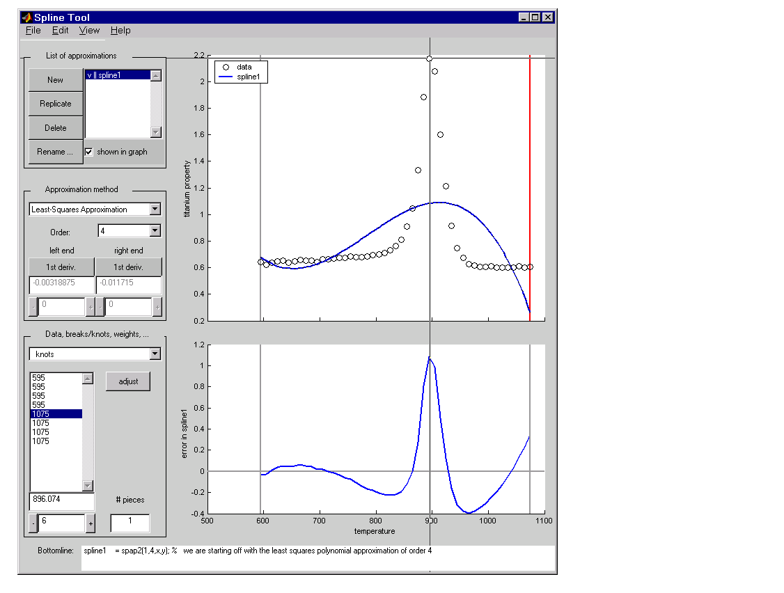
Notice how poorly this approximates the data since there are no interior knots. To view the current knots and add new knots, choose knots from Data, breaks/knots, weights. The knots are now listed in knots, and also displayed in the data graph as vertical lines. Notice that there are just the two end knots, each with multiplicity 4.
Right-click in the data graph and choose Add Knot. This brings up crosshairs for you to move with the mouse. Its precise horizontal location is shown in the edit field below the list of knots. A mouse click places a new knot at the current location of the crosshairs. One possible strategy is to place the additional knot at the place of maximum absolute error, as shown in the auxiliary graph below.

If you right-click and choose Replicate Knot, you will increase the multiplicity of the current knot, which is shown by its repeated occurrence in knots. If you don't like a particular knot, you can delete it. To delete a specific knot, you must first select it in either the list of knots or the data graph, and then right-click in the graph and choose Delete Knot.

You could also ask for an approximation using six polynomial pieces, which corresponds to five interior knots. To do this, enter 6 as # pieces in Data, breaks/knots, weights.
After you have the five interior knots, try to make the error even smaller by moving the knots. To do this, select the knot you want to move by clicking on its vertical line in the graph, then use the interface control below knots in Data, breaks/knots, weights and observe how the error changes with the movement of the knot. You can also use the edit field to overwrite the current knot location. You could also try adjust, which redistributes the current knot sequence.
Use Replicate in List of approximations to save any good knot distribution for later use. Rename the replicated approximation to lstsqr using Rename. To return to the original approximation, click on its name in List of Approximations.

Smoothing Spline

This example experiments with smoothing splines:

Type splinetool at the command line or, if the GUI is already running, click on File->Restart.
Choose Titanium heat data.
In Approximation method, choose Smoothing Spline.
Vary parameter between 0 and 1, which changes the approximation from the least-squares straight-line approximation to the "natural" cubic spline interpolant.
Vary tolerance between 0 and some large value, even inf. The approximation changes from the best possible one, the "natural" cubic spline interpolant, to the least-squares straight-line approximation.
As you increase the parameter value or decrease the tolerance value, the error decreases. However, a smaller error corresponds to more roughness, as measured by the size of the second derivative. To see this, choose View->Show 2nd Derivative and vary the parameter and tolerance values once again.
This step modifies the weights in the error measure to force the approximation to pass through a particular data point.

Set tolerance to 0.2. Notice that the approximation does not pass through the highest data point. To see the large error at this site, choose View->Error.
To force the smoothing spline to go through this point, choose sites and error weights from Data, breaks/knots, weights.
Click on the highest data point in the graph and notice its site, which is indicated in the sites list box.
Use the edit field beneath the list of weights to change the current weight to 1000. Notice how much closer the smoothing spline now comes to that highest data point, and the decrease in the error at that site.

This step modifies the weights in the roughness measure to force the approximation to balance the error with the smoothness of the second derivative.

Choose sites and roughness weight from Data, breaks/knots, weights.
Choose View->Show 2nd Derivative
Select any data point to the left of the peak in the data.
Set the jump across the selected site to -1 by changing its value in the edit field below it. Since the roughness weight for the very first site interval is 1, you have just set the roughness weight to the right of the highlighted site to 0. Correspondingly, the second derivative has become relatively small to the left of that site.
Select any data point to the right of the peak in the data.
Set the jump across the selected site to 1. Since the roughness weight just to the left of the highlighted site is 0, you have just set the roughness weight to the right of the highlighted site to 1. Correspondingly, the second derivative has become relatively small to the right of that site. The total effect is a very smooth but not very accurate fit away from the peak, while in the peak area, the spline fit is much better but the second derivative is much larger.

At the sites where there is a jump in the roughness weight, there is a corresponding jump in the second derivative. If you increase the parameter value, the error across the peak area decreases but the second derivative remains quite large, while the opposite holds true away from the peak area.

See Also

csape, csapi, csaps, spap2, spapi, spaps

spcrv splpp, sprpp