Curve Fitting Toolbox

The Least Squares Fitting Method

The Curve Fitting Toolbox uses the method of least squares when fitting data. The fitting process requires a model that relates the response data to the predictor data with one or more coefficients. The result of the fitting process is an estimate of the "true" but unknown coefficients of the model.

To obtain the coefficient estimates, the least squares method minimizes the summed square of residuals. The residual for the ith data point r_i is defined as the difference between the observed response value y_i and the fitted response value , and is identified as the error associated with the data.

The summed square of residuals is given by

where n is the number of data points included in the fit and S is the sum of squares error estimate. The supported types of least squares fitting include

• Linear least squares
• Weighted linear least squares
• Robust least squares
• Nonlinear least squares

Linear Least Squares

The Curve Fitting Toolbox uses the linear least squares method to fit a linear model to data. A linear model is defined as an equation that is linear in the coefficients. For example, polynomials are linear but Gaussians are not. To illustrate the linear least squares fitting process, suppose you have n data points that can be modeled by a first-degree polynomial.

To solve this equation for the unknown coefficients p₁ and p₂, you write S as a system of n simultaneous linear equations in two unknowns. If n is greater than the number of unknowns, then the system of equations is overdetermined.

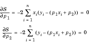
Because the least squares fitting process minimizes the summed square of the residuals, the coefficients are determined by differentiating S with respect to each parameter, and setting the result equal to zero.

The estimates of the true parameters are usually represented by b. Substituting b₁ and b₂ for p₁ and p₂, the previous equations become

where the summations run from i =1 to n. The normal equations are defined as

Solving for b₁

Solving for b₂ using the b₁ value

As you can see, estimating the coefficients p₁ and p₂ requires only a few simple calculations. Extending this example to a higher degree polynomial is straightforward although a bit tedious. All that is required is an additional normal equation for each linear term added to the model.

In matrix form, linear models are given by the formula

where

• y is an n-by-1 vector of responses.
• is a m-by-1 vector of coefficients.
• X is the n-by-m design matrix for the model.
• is an n-by-1 vector of errors.

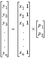
For the first-degree polynomial, the n equations in two unknowns are expressed in terms of y, X, and as

The least squares solution to the problem is a vector b, which estimates the unknown vector of coefficients . The normal equations are given by

where X^T is the transpose of the design matrix X. Solving for b,

In MATLAB, you can use the backslash operator to solve a system of simultaneous linear equations for unknown coefficients. Because inverting X^TX can lead to unacceptable rounding errors, MATLAB uses QR decomposition with pivoting, which is a very stable algorithm numerically. Refer to Arithmetic Operators in the MATLAB documentation for more information about the backslash operator and QR decomposition.

You can plug b back into the model formula to get the predicted response values, .

A hat (circumflex) over a letter denotes an estimate of a parameter or a prediction from a model. The projection matrix H is called the hat matrix, because it puts the hat on y.

The residuals are given by

Refer to [1] or [2] for a complete description of the matrix representation of least squares regression.

Weighted Linear Least Squares

As described in Basic Assumptions About the Error, it is usually assumed that the response data is of equal quality and, therefore, has constant variance. If this assumption is violated, your fit might be unduly influenced by data of poor quality. To improve the fit, you can use weighted least squares regression where an additional scale factor (the weight) is included in the fitting process. Weighted least squares regression minimizes the error estimate

where w_i are the weights. The weights determine how much each response value influences the final parameter estimates. A high-quality data point influences the fit more than a low-quality data point. Weighting your data is recommended if the weights are known, or if there is justification that they follow a particular form.

The weights modify the expression for the parameter estimates b in the following way,

where W is given by the diagonal elements of the weight matrix w.

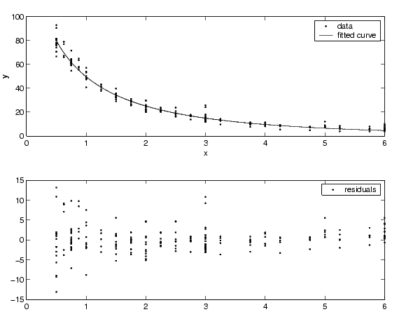
You can often determine whether the variances are not constant by fitting the data and plotting the residuals. In the plot shown below, the data contains replicate data of various quality and the fit is assumed to be correct. The poor quality data is revealed in the plot of residuals, which has a "funnel" shape where small predictor values yield a bigger scatter in the response values than large predictor values.

The weights you supply should transform the response variances to a constant value. If you know the variances of your data, then the weights are given by

If you don't know the variances, you can approximate the weights using an equation such as

This equation works well if your data set contains replicates. In this case, n is the number of sets of replicates. However, the weights can vary greatly. A better approach might be to plot the variances and fit the data using a sensible model. The form of the model is not very important -- a polynomial or power function works well in many cases.

Robust Least Squares

As described in Basic Assumptions About the Error, it is usually assumed that the response errors follow a normal distribution, and that extreme values are rare. Still, extreme values called outliers do occur.

The main disadvantage of least squares fitting is its sensitivity to outliers. Outliers have a large influence on the fit because squaring the residuals magnifies the effects of these extreme data points. To minimize the influence of outliers, you can fit your data using robust least squares regression. The toolbox provides these two robust regression schemes:

• Least absolute residuals (LAR) -- The LAR scheme finds a curve that minimizes the absolute difference of the residuals, rather than the squared differences. Therefore, extreme values have a lesser influence on the fit.
• Bisquare weights -- This scheme minimizes a weighted sum of squares, where the weight given to each data point depends on how far the point is from the fitted line. Points near the line get full weight. Points farther from the line get reduced weight. Points that are farther from the line than would be expected by random chance get zero weight.

• For most cases, the bisquare weight scheme is preferred over LAR because it simultaneously seeks to find a curve that fits the bulk of the data using the usual least squares approach, and it minimizes the effect of outliers.

Robust fitting with bisquare weights uses an iteratively reweighted least squares algorithm, and follows this procedure:

1. Fit the model by weighted least squares.
2. Compute the adjusted residuals and standardize them. The adjusted residuals are given by

1. r_i are the usual least squares residuals and h_i are leverages that adjust the residuals by downweighting high-leverage data points, which have a large effect on the least squares fit. The standardized adjusted residuals are given by

1. K is a tuning constant equal to 4.685, and s is the robust variance given by MAD/0.6745 where MAD is the median absolute deviation of the residuals. Refer to [7] for a detailed description of h, K, and s.

3. Compute the robust weights as a function of u. The bisquare weights are given by

1. Note that if you supply your own regression weight vector, the final weight is the product of the robust weight and the regression weight.

4. If the fit converges, then you are done. Otherwise, perform the next iteration of the fitting procedure by returning to the first step.

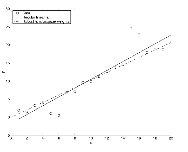
The plot shown below compares a regular linear fit with a robust fit using bisquare weights. Notice that the robust fit follows the bulk of the data and is not strongly influenced by the outliers.

Instead of minimizing the effects of outliers by using robust regression, you can mark data points to be excluded from the fit. Refer to Excluding and Sectioning Data for more information.

Nonlinear Least Squares

The Curve Fitting Toolbox uses the nonlinear least squares formulation to fit a nonlinear model to data. A nonlinear model is defined as an equation that is nonlinear in the coefficients, or a combination of linear and nonlinear in the coefficients. For example, Gaussians, ratios of polynomials, and power functions are all nonlinear.

In matrix form, nonlinear models are given by the formula

where

• y is an n-by-1 vector of responses.
• f is a function of and X.
• is a m-by-1 vector of coefficients.
• X is the n-by-m design matrix for the model.
• is an n-by-1 vector of errors.

Nonlinear models are more difficult to fit than linear models because the coefficients cannot be estimated using simple matrix techniques. Instead, an iterative approach is required that follows these steps:

1. Start with an initial estimate for each coefficient. For some nonlinear models, a heuristic approach is provided that produces reasonable starting values. For other models, random values on the interval [0,1] are provided.
2. Produce the fitted curve for the current set of coefficients. The fitted response value is given by

• and involves the calculation of the Jacobian of f(X,b), which is defined as a matrix of partial derivatives taken with respect to the coefficients.

3. Adjust the coefficients and determine whether the fit improves. The direction and magnitude of the adjustment depend on the fitting algorithm. The toolbox provides these algorithms:
• Trust-region -- This is the default algorithm and must be used if you specify coefficient constraints. It can solve difficult nonlinear problems more efficiently than the other algorithms and it represents an improvement over the popular Levenberg-Marquardt algorithm.
• Levenberg-Marquardt -- This algorithm has been used for many years and has proved to work most of the time for a wide range of nonlinear models and starting values. If the trust-region algorithm does not produce a reasonable fit, and you do not have coefficient constraints, you should try the Levenberg-Marquardt algorithm.
• Gauss-Newton -- This algorithm is potentially faster than the other algorithms, but it assumes that the residuals are close to zero. It's included with the toolbox for pedagogical reasons and should be the last choice for most models and data sets.

1. For more information about the trust region algorithm, refer to [4] and to Trust Region Methods for Nonlinear Minimization in the Optimization Toolbox documentation. For more information about the Levenberg-Marquardt and Gauss-Newton algorithms, refer to Nonlinear Least Squares Implementation in the same guide. Additionally, the Levenberg-Marquardt algorithm is described in [5] and [6].

4. Iterate the process by returning to step 2 until the fit reaches the specified convergence criteria.

You can use weights and robust fitting for nonlinear models, and the fitting process is modified accordingly.

Because of the nature of the approximation process, no algorithm is foolproof for all nonlinear models, data sets, and starting points. Therefore, if you do not achieve a reasonable fit using the default starting points, algorithm, and convergence criteria, you should experiment with different options. Refer to Specifying Fit Options for a description of how to modify the default options. Because nonlinear models can be particularly sensitive to the starting points, this should be the first fit option you modify.

Basic Assumptions About the Error

Library Models