Curve Fitting Toolbox

Specifying Fit Options

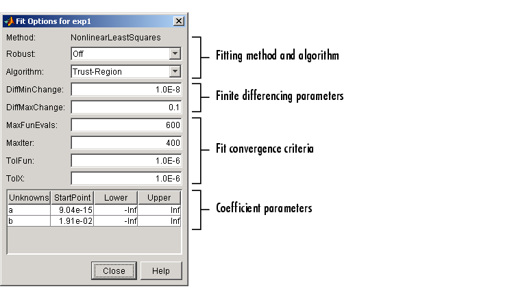
You specify fit options with the Fit Options GUI. The fit options for the single-term exponential are shown below. The coefficient starting values and constraints are for the census data.

The available GUI options depend on whether you are fitting your data using a linear model, a nonlinear model, or a nonparametric fit type. All the options described below are available for nonlinear models. Method, Robust, and coefficient constraints (Lower and Upper) are available for linear models. Interpolants and smoothing splines include Method, but no configurable options.

Fitting Method and Algorithm

• Method -- The fitting method.

• The method is automatically selected based on the library or custom model you use. For linear models, the method is LinearLeastSquares. For nonlinear models, the method is NonlinearLeastSquares.

• Robust -- Specify whether to use the robust least squares fitting method. The values are
• Off -- Do not use robust fitting (default).
• On -- Fit with default robust method (bisquare weights).
• LAR -- Fit by minimizing the least absolute residuals (LAR).
• Bisquare -- Fit by minimizing the summed square of the residuals, and downweight outliers using bisquare weights. In most cases, this is the best choice for robust fitting.
• Algorithm -- Algorithm used for the fitting procedure:
• Trust-Region -- This is the default algorithm and must be used if you specify coefficient constraints.
• Levenberg-Marquardt -- If the trust-region algorithm does not produce a reasonable fit, and you do not have coefficient constraints, you should try the Levenberg-Marquardt algorithm.
• Gauss-Newton -- This algorithm is included for pedagogical reasons and should be the last choice for most models and data sets.

Finite Differencing Parameters

• DiffMinChange -- Minimum change in coefficients for finite difference Jacobians. The default value is 10^-8.
• DiffMaxChange -- Maximum change in coefficients for finite difference Jacobians. The default value is 0.1.

Fit Convergence Criteria

• MaxFunEvals -- Maximum number of function (model) evaluations allowed. The default value is 600.
• MaxIter -- Maximum number of fit iterations allowed. The default value is 400.
• TolFun -- Termination tolerance used on stopping conditions involving the function (model) value. The default value is 10^-6.
• TolX -- Termination tolerance used on stopping conditions involving the coefficients. The default value is 10^-6.

Coefficient Parameters

• Unknowns -- Symbols for the unknown coefficients to be fitted.
• StartPoint -- The coefficient starting values. The default values depend on the model. For rational, Weibull, and custom models, default values are randomly selected within the range [0,1]. For all other nonlinear library models, the starting values depend on the data set and are calculated heuristically.
• Lower -- Lower bounds on the fitted coefficients. The bounds are used only with the trust region fitting algorithm. The default lower bounds for most library models are -Inf, which indicates that the coefficients are unconstrained. However, a few models have finite default lower bounds. For example, Gaussians have the width parameter constrained so that it cannot be less than 0.
• Upper -- Upper bounds on the fitted coefficients. The bounds are used only with the trust region fitting algorithm. The default upper bounds for all library models are Inf, which indicates that the coefficients are unconstrained.

For more information about these fit options, refer to Optimization Options Parameters in the Optimization Toolbox documentation.

Default Coefficient Parameters

The default coefficient starting points and constraints for library and custom models are given below. If the starting points are optimized, then they are calculated heuristically based on the current data set. Random starting points are defined on the interval [0,1] and linear models do not require starting points.

If a model does not have constraints, the coefficients have neither a lower bound nor an upper bound. You can override the default starting points and constraints by providing your own values using the Fit Options GUI.

Table 3-1: Default Starting Points and Constraints

Model	Starting Points	Constraints
Custom linear	N/A	None
Custom nonlinear	Random	None
Exponentials	Optimized	None
Fourier series	Optimized	None
Gaussians	Optimized	ci > 0
Polynomials	N/A	None
Power series	Optimized	None
Rationals	Random	None
Sum of sines	Optimized	bi > 0
Weibull	Random	a, b > 0

Note that the sum of sines and Fourier series models are particularly sensitive to starting points, and the optimized values might be accurate for only a few terms in the associated equations. For an example that overrides the default starting values for the sum of sines model, refer to Example: Sectioning Periodic Data.

Custom Equations

Evaluating the Goodness of Fit