Synchronous Machine (SimPowerSystems)

Model the dynamics of a three-phase round rotor or salient-pole synchronous machine

Library

Machines

Description

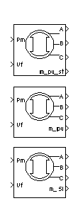
The Synchronous Machine block operates in generating or motoring modes. The operating mode is dictated by the sign of the mechanical power (positive for generating, negative for motoring). The electrical part of the machine is represented by a sixth-order state-space model and the mechanical part is the same as in the Simplified Synchronous Machine block.

The model takes into account the dynamics of the stator, field, and damper windings. The equivalent circuit of the model is represented in the rotor reference frame (qd frame). All rotor parameters and electrical quantities are viewed from the stator. They are identified by primed variables. The subscripts used are defined as follows:

d,q: d and q axis quantity
R,s: Rotor and stator quantity
l,m: Leakage and magnetizing inductance
f,k: Field and damper winding quantity

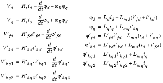
The electrical model of the machine is

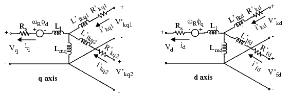
with the following equations.

Dialog Box and Parameters

In the powerlib library you can choose among three Synchronous Machine blocks to specify the parameters of the model.

Fundamental Parameters in SI Units

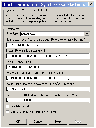
Rotor type: Specifies rotor type: salient-pole or round (cylindrical). This choice affects the number of rotor circuits in the q-axis (damper windings).
Nominal: The total three-phase apparent power Pn (VA), rms line-to-line voltage Vn (V), frequency fn (Hz), and field current ifn (A).

The nominal field current is the current that produces nominal terminal voltage under no-load conditions. This model was developed with all quantities viewed from the stator. The nominal field current makes it possible to compute the transformation ratio of the machine, which allows you to apply the field voltage viewed from the rotor, as in real life. This also allows the field current, which is a variable in the output vector of the model, to be viewed from the rotor. If the value of the nominal field current is not known, you must enter 0. Since the transformation ratio cannot be determined in this case, you have to apply the field voltage as viewed from the stator and the field current in the output vector is also viewed from the stator.
Stator: The resistance Rs (), leakage inductance Lls (H), and d-axis and q-axis magnetizing inductances Lmd (H) and Lmq (H).
Field: The field resistance Rf' () and leakage inductance Llfd' (H), both referred to the stator.
Dampers: The d-axis resistance Rkd' () and leakage inductance Llkd' (H), the q-axis resistance Rkq1' () and leakage inductance Llkq1' (H), and (if round rotor only) the q-axis resistance Rkq2' () and leakage inductance Llkq2' (H). All these values are referred to the stator.
Mechanical: The inertia coefficient J (kg.m²), damping coefficient D (N.m.s./rad), and number of pole pairs p.
Initial conditions: The initial speed deviation (% of nominal speed), electrical angle of the rotor e (deg), line current magnitudes ia, ib, ic (A) and phase angles pha, phb, phc (deg), and the initial field voltage Vf (V).

You can specify the initial field voltage in one of two ways. If you know the nominal field current (first line, last parameter) enter in the dialog box the initial field voltage in volts DC referred to the rotor. Otherwise, enter a 0 as nominal field current, as explained earlier, and specify the initial field voltage in volts DC referred to the stator. You can easily determine the nominal field voltage viewed from the stator by selecting the Display Vfd which produces a nominal Vt check box at the bottom of the dialog box.
Simulate saturation: Specifies whether magnetic saturation of rotor and stator iron is to be simulated or not.
Saturation: The no-load saturation curve parameters. Magnetic saturation of stator and rotor iron is modeled by a nonlinear function, in this case a polynomial, using points on the no-load saturation curve. You must enter a 2-by-n matrix, where n is the number of points taken from the saturation curve. The first row of this matrix contains the values of field currents, while the second row contains values of corresponding terminal voltages. The first point (first column of the matrix) must correspond to the point where the effect of saturation begins. You must select the Simulate saturation check box to simulate saturation. This check box allows you to enter the matrix of parameters for simulating the saturation. If you do not want to model saturation in your simulation, simply do not select the Simulate saturation check box. In this case the relationship between ifd and Vt obtained is linear (no saturation).; As an example, without saturation, a typical curve might be as shown below. Here ifn is 1087 A and Vn is 13800 V rms line-to-line, which is also 11268 V peak line-to-neutral.

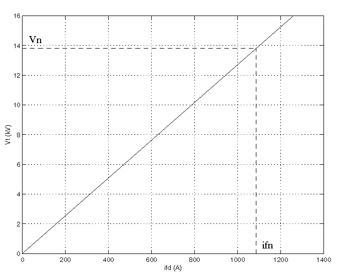
When saturation is modeled, a polynomial is fitted to the curve corresponding to the matrix of points you enter. The more points you enter, the better the fit to the original curve.

The next figure illustrates this graphically (the diamonds are the actual points entered in the dialog box).

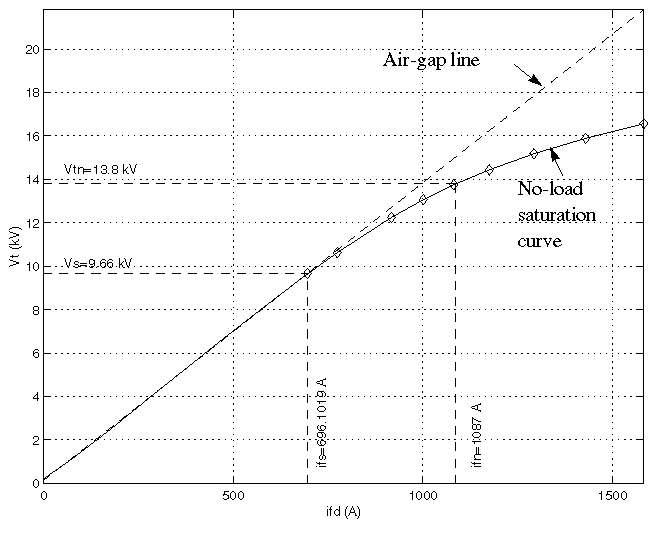
In this particular case, the following values were used:

ifn = 1087 A
ifd = [695.64, 774.7, 917.5, 1001.6, 1082.2, 1175.9, 1293.6, 1430.2, 1583.7] A
Vt = [9660, 10623, 12243, 13063, 13757, 14437, 15180, 15890, 16567] V

Fundamental Parameters in p.u.

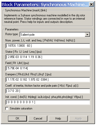
Rotor type: Specifies rotor type: salient-pole or round (cylindrical).
Nominal: Total three-phase apparent power (VA), rms line-to-line voltage (V), frequency (Hz), and field current (A).; This line is identical to the first line of the fundamental parameters in SI dialog box, except that you do not specify a nominal field current. This value is not required here because we do not need the transformation ratio. Since rotor quantities are viewed from the stator, they are converted to p.u. using the stator base quantities derived from the preceding three nominal parameters.
Stator, field and dampers: Contain exactly the same parameters as in the previous dialog box, but they are expressed here in p.u. instead of SI units.
Mechanical: The inertia constant H (s), where H is the ratio of energy stored in the rotor at nominal speed over the nominal power of the machine, the damping coefficient D (p.u. torque/p.u. speed deviation), and the number of pole pairs p.
Initial conditions, Simulate saturation, Saturation

The same initial conditions and saturation parameters as in the S.I. units dialog box, but all values are expressed in p.u. instead of SI units. For saturation, the nominal field current multiplied by the d-axis magnetizing inductance and nominal rms line-to-line voltage are the base values for the field current and terminal voltage, respectively.

Standard Parameters in p.u.

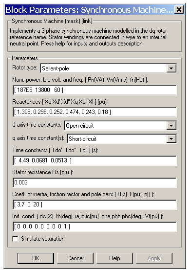
Rotor type, Nominal: The same parameters as the fundamental p.u. dialog box.
Reactances: The d-axis synchronous reactance Xd, transient reactance Xd', and subtransient reactance Xd'', the q-axis synchronous reactance Xq, transient reactance Xq' (only if round rotor), and subtransient reactance Xq'', and finally the leakage reactance Xl (all in p.u.).
d-axis time constants, q-axis time constant(s): Specify which time constants you supply for each axis: either open-circuit or short-circuit.
Time constants: The d-axis and q-axis time constants (all in s). These values must be consistent with choices made on the two previous lines: d-axis transient open-circuit (Tdo') or short-circuit (Td') time constant, d-axis subtransient open-circuit (Tdo'') or short-circuit (Td'') time constant, q-axis transient open-circuit (Tqo') or short-circuit (Tq') time constant (only if round rotor), q-axis subtransient open-circuit (Tqo'') or short-circuit (Tq'') time constant.
Stator resistance: The stator resistance Rs (p.u.).
Mechanical, Initial conditions, Simulate saturation, Saturation: The same parameters as the fundamental parameters in p.u. dialog box.

Note These three blocks simulate exactly the same Synchronous machine model; the only difference is the way of entering the parameter units.

Inputs and Outputs

The units of inputs and outputs vary according to which dialog box was used to enter the block parameters. For the nonelectrical connections, there are two possibilities. If the first dialog box (fundamental parameters in SI units) is used, the inputs and outputs are in SI units (except for dw in the vector of internal variables, which is always in p.u., and angle , which is always in rad). If the second or third dialog boxes is used, the inputs and outputs are in p.u.

The first input is the mechanical power at the machine's shaft. In generating mode, this input can be a positive constant or function or the output of a prime mover block (see the Hydraulic Turbine and Governor or Steam Turbine and Governor blocks). In motoring mode, this input is usually a negative constant or function.

The second input of the block is the field voltage and can be supplied by a voltage regulator (see the Excitation System block) in generating mode and is usually a constant in motoring mode.

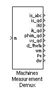
The first three outputs are the electrical terminals of the stator. The last output of the block is a vector containing 16 variables. They are, in order:

1-3: Stator currents (flowing out of machine) i_sa, i_sb, and i_sc
4-5: q- and d-axis stator currents (flowing out of machine) i_q, i_d
6-8: Field and damper winding currents (flowing into machine)
i_fd, i_kq, and i_kd
9-10: q- and d-axis magnetizing fluxes _mq, _md
11-12: q- and d-axis stator voltages v_q,v_d
13: Rotor angle deviation , also known as power angle
14: Rotor speed _r
15: Electrical power Pe
16: Rotor speed deviation dw

You can demultiplex these variables by using the special Machines Measurement Demux block provided in the Machines library.

Example

The psbsyncmachine.mdl demo illustrates the use of the Synchronous Machine block in motoring mode. The simulated system consists of an industrial grade synchronous motor (150 HP, 440V) connected to an infinite bus. After the machine reaches a stable speed, the load (mechanical power) is changed from 50 kW to 60 kW. The initial conditions are set in such a way that the simulation starts in steady state.

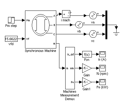
Set the simulation parameters as follows:

Integrator type: Stiff, ode15s
Stop time: 5 s
Integration options: Use default settings, except for Max. step size, which you must set to 0.005 s

Run the simulation and observe the speed, power, and current of the motor.

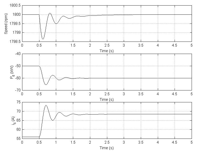
Since this is a four pole machine, the nominal speed is 1800 rpm. The initial speed is 1800 rpm as prescribed (top graph). The load passes from 50 kW to 60 kW at t=0.5 s. The machine then oscillates before stabilizing to 1800 rpm.

Now, look at the electrical power (middle graph). Since we are in motoring mode, the machine absorbs power and Pe is negative. As expected, the power starts at -50 kW until the load is changed at t = 0.5 seconds, at which point the power oscillates before settling at -60 kW.

Finally, look at the stator current i_s. As expected, the current starts with the value corresponding to a three-phase power of 50 kW (56 A), before oscillating and settling to the value corresponding to a 60 kW load (68.5 A).

References

[1] Krause P.C., Analysis of Electric Machinery, McGraw-Hill, 1986, Section 12.5.

[2] Kamwa I. et al., "Experience with Computer-Aided Graphical Analysis of Sudden-Short-Circuit Oscillograms of Large Synchronous Machines," IEEE Transactions on Energy Conversion, Vol.10, No.3, September 1995.

Synchronized 12-Pulse Generator 3-Phase Breaker