| SimMechanics | |
Adding Sensors and Starting the Simulation
To measure the motion of the pendulum as it swings, you need to hook one or more Simulink Scope blocks to your model. The special library of Actuators and Sensor blocks gives you the means to input and output Simulink signals to and from SimMechanics models. Sensors allow you to watch the mechanical motion once you start the simulation, as the following explain:
Connecting and Configuring Pendulum Sensors
In this example, you measure the angular motion of the revolute joint:
0 to 2 using the spinner menu. Two open connector ports  appear on either side of Revolute. Close Revolute.
 .
.
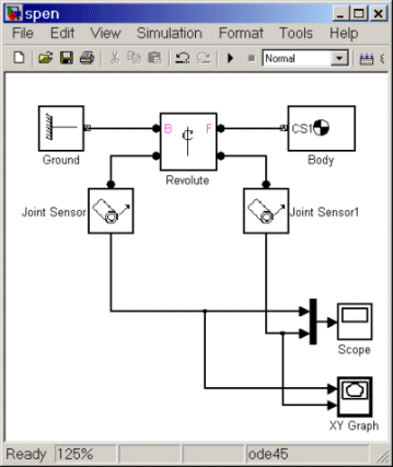
> to the Scope and XY Graph blocks are normal Simulink signal lines and can be branched. You cannot branch the lines connecting SimMechanics blocks to each another at the round connector ports  .
.
spen.mdl.
You now need to configure the global parameters of your model before you can run it.
Configuring Simulation Parameters and Mechanical Environment Settings
The Simulation Parameters dialog box is a standard feature of Simulink. Reset its entries for this model to obtain more accurate simulation results.
1e-6 and Absolute tolerance to 1e-4.
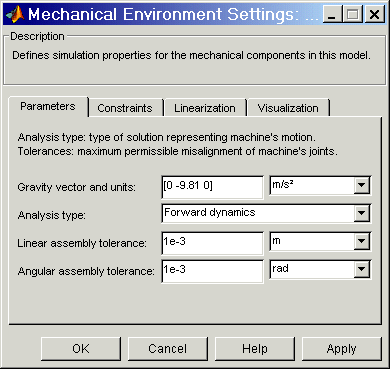
A special feature of SimMechanics models is the Mechanical Environment Settings dialog box.
[0 -9.81 0] m/s2, which points in the -y direction, as shown in Figure 2-2. Gravitational acceleration g = 9.81 m/s2.
Starting and Interpreting the Motion
You can now start your simulation and watch the pendulum motion via the Scope and XY Graph blocks:
| Parameter |
Value |
x-min |
0 |
x-max |
200 |
y-min |
-500 |
y-max |
500 |
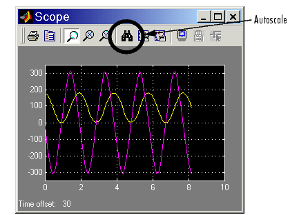
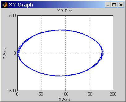
Angle and Angular Velocity of the Simple Pendulum as Functions of Time
The XY Graph shows the angle versus angular velocity, with no explicit time axis. These two variables trace out a figure similar to an ellipse, because of the conservation of total energy E:
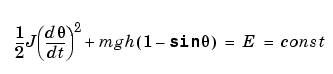
where J = Izz + mL2/4 is the inertial moment of the rod about its pivot point (not the center of gravity). The two terms on the left side of this equation are the kinetic and potential energies, respectively. The coordinate-velocity space is the phase space of the system.
Phase Space Plot of Simple Pendulum Motion: Angular Velocity Versus Angle
The directionality of the Revolute Joint assumes that the rotation axis lies in the +z direction. Looking at the pendulum from the front, follow Figure 2-1, Figure 2-2, and Figure 2-3. Positive angular motion from this perspective is counterclockwise, following the right-hand rule.
The next tutorial walks you through visualizing and animating this same simple pendulum model.
| | Configuring a Joint Block | Visualizing a Simple Pendulum | |