Model Predictive Control Toolbox

Model predictive controller for simulating closed-loop systems with saturation constraints on the manipulated variables using linear models in the MPC step format for nonlinear plants represented as Simulink S-functions.

Description
nlmpcsim is a Simulink S-function block and can be invoked by typing nlmpclib at the MATLAB prompt. Its usage is identical to other Simulink blocks. The input to nlmpcsim includes both the variables controlled by nlmpcsim and measured disturbances. The first ny elements of the input are treated as the controlled variables while the rest is taken as the measured disturbances. The output from nlmpcsim are the values of the manipulated variables. Initial conditions for the manipulated variables and the measured disturbances must be specified. Both the controlled variables sent to nlmpcsim and the manipulated variables returned by nlmpcsim are the actual variables; they are not deviation variables.

Because of the limit on the number of masked variables that can be specified for a Simulink block, model and dmodel are put together as one variable. u0 and d0 should be entered as one row vector. The required input variables are as follows:

modelpd
Equals [model dmodel]. model is a linear model in the MPC step format that is to be used for state estimation in the controller. In general, it is a linear approximation for the nonlinear plant. Note, however, that model should be the same as that used to calculate Kmpc. dmodel is a model in MPC step format representing the measured disturbances. If dmodel = [ ], the default is no measured disturbances. Note that the truncation time for model and dmodel should be the same and the number of outputs for model and dmodel should be the same.

r

Kmpc
Is the MPC controller gain matrix, usually calculated using the function mpccon.

r
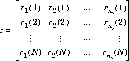
Is a setpoint matrix consisting of N rows and ny columns, where ny is the number of controlled variables, y:

Where ri(k) is the setpoint for output i at time t = kT, and T is the sampling period (as specified in the step format of model). If the simulation time is larger than NT, the setpoints vary for the first N periods in the simulation, as specified by r, and are then held constant at the values given in the last row of r for the remainder of the simulation.

In many simulations one wants the setpoints to be constant for the entire time, in which case r need only contain a single row of ny values.

Note that r is the actual setpoint. If you set r=[ ], the default is y0.

usat
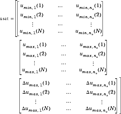
Is a matrix giving the saturation limits on the manipulated variables. Its format is as follows:

Note that it contains three matrices of N rows. N may be different from that for the setpoint matrix, r, but the idea is the same: the saturation limits will vary for the first N sampling periods of the simulation, then be held constant at the values given in the last row of usat for the remaining periods (if any).

The first matrix specifies the lower bounds on the nu manipulated variables. For example, umin,j(k) is the lower bound for manipulated variable j at time t = kT in the simulation. If umin,j(k) = -inf, manipulated variable j will have no lower bound at t = kT.

The second matrix gives the upper bounds on the manipulated variables. If umax,j(k) = inf, manipulated variable j will have no upper bound at t = kT.

The lower and upper bounds may be either positive or negative (or zero) as long as umin,j(k) umax,j(k).

The third matrix gives the limits on the rate of change of the manipulated variables. In other words, mpcsim will force|uj(k) - uj(k - 1)| umax,j(k). The limits on the rate of change must be nonnegative.

If usat = [ ], then all the umin values will be set to -inf, and all the umax and umax values will be set to inf.

Note: Saturation constraints are enforced by simply clipping the manipulated variable moves so that they satisfy all constraints. This is a nonoptimal solution that, in general, will differ from the results you would get using the ulim variable in cmpc or nlcmpc.

tfilter
Is a matrix of time constants for the noise filter and the unmeasured disturbances entering at the plant output. The first row of ny elements gives the noise filter time constants and the second row of ny elements gives the time constants of the lags through which the unmeasured disturbance steps pass. If tfilter only contains one row, the unmeasured disturbances are assumed to be steps. If you set tfilter= [ ], no noise filtering and steplike unmeasured disturbances are assumed.

ud0
Equals [u0 d0]. u0 are initial values of the manipulated variables arranged in a row vector having nu elements; nu is the number of the manipulated variables computed by nlmpcsim. d0 are initial values of the measured disturbances arranged in a row vector having nd elements; nd is the number of the measured disturbances. The default is u0 = 0 and d0 = 0.

Note:
You may use a different number of rows in the matrices r and usat, should that be appropriate for your simulation.

Examples
Let us now demonstrate the use of the controller nlmpcsim. Since the plant used in Example 1 is linear, using mpcsim would be much faster. The point, however, is to show how masked variables are specified for nlmpcsim.

   1.

The plant is linear with two inputs and two outputs. It is represented by

Figure 1-1 Simulink Block for Example 1

• g11=poly(0.4,[1 2]);
  g21=poly2tfd(0,1);
  g12=poly2tfd(0,1);
  g22=poly2tfd(1,[1 1]);
  tfinal=8;
  delt=0.2;
  nout=2;
  model=tfd2step(tfinal,delt,nout,g11,g21,g12,g22);
  ywt=[1 1];
  uwt=[0 0];
  M=4;
  P=10;
  r=[68.3 2];
  usat=[100 1 200 3 200 200];
  tfilter=[ ];
  Kmpc = mpccon(model,ywt,uwt,M,P);
  dmodel = [ ];
  

• plant='nlmpcdm1'; y0=[58.3 1.5];
  u0=[100 1];
  tfsim = 2;
  tol=[1e-3];
  minstep=[ ];
  maxstep=[ ];
  [t,yu]=gear(plant,tfsim,[y0 u0],[tol,minstep,maxstep]);
  

Figure 1-2 Output responses for a setpoint change for Example 1

   2.

The plant is the paper machine headbox discussed in the section, "Application: Paper Machine Headbox Control" in Chapter 3. The nonlinear plant model is represented as a Simulink S-function and is in pap_mach.m. The plant has two inputs, three outputs, four states, one measured disturbance, and one unmeasured disturbance. All these variables are zero at the nominal steady-state. Since the model for nlmpcsim must be linear, we linearize the nonlinear plant at the nominal steady-state to obtain a linear model. Since the model is simple, we can linearize it analytically to obtain A, B, C, and D.

The Simulink block to simulate this nonlinear plant using nlmpcsim is in nlmpcdm2.m and shown in Figure 1-3.

Figure 1-3 Simulink Block for Example 2

• A=[-1.93 0 0 0; .394 -.426 0 0; 0 0 -.63 0; .82 -.784 
      .413 -.426];
  B=[1.274 1.274 0; 0 0 0; 1.34 -.65 .203; 0 0 0];
  C=[0 1 0 0; 0 0 1 0; 0 0 0 1];
  D=zeros(3,3);
  % Discretize the linear model and save in MOD form. 
  dt=2;
  [PHI,GAM]=c2dmp(A,B,dt);
  minfo=[dt,4,2,1,0,3,0];
  imod=ss2mod(PHI,GAM,C,D,minfo);
  % Store plant model and measured disturbance model in MPC 
  % step format
  [model,dmodel]=mod2step(imod,20);
  m=5;
  p=20;
  ywt=[1 0 5]; % unequal weighting of y1 and y3, no control 
  % of y2 
  uwt=[1 1]; % Equal weighting of u1 and u2 
  ulim=[-10 -10 10 10 2 2]; % Constraints on u 
  ylim=[ ]; % No constraints on y 
  usat=ulim;
  tfilter=[ ];
  y0=[0 0 0];
  u0=[0 0];
  r=[0 0 0];
  Kmpc=mpccon(model,ywt,uwt,M,P);
  

Figure 1-4 Output responses for a unit-step measured disturbance Np = 1 and a step unmeasured disturbance Nw = 5

See Also