Model Predictive Control Toolbox

Simulates closed-loop systems with saturation constraints on the manipulated variables using models in the MPC step format. Can also be used for open-loop simulations.

Syntax

• yp = mpcsim(plant,model,Kmpc,tend,r) 
  [yp,u,ym] = mpcsim(plant,model,Kmpc,tend,r,usat,...
     tfilter,dplant,dmodel,dstep) 
  
  

Description

mpcsim provides a convenient way to simulate the performance of the type of system shown in the above diagram. Measurement noise can be simulated by treating it as an unmeasured disturbance. The required input variables are as follows:

plant
Is a model in the MPC step format that is to represent the plant.

model
Is a model in the MPC step format that is to be used for state estimation in the controller. In general, it can be different from plant if you want to simulate the effect of plant/controller model mismatch. Note, however, that model should be the same as that used to calculate Kmpc.

Kmpc
Is the MPC controller gain matrix, usually calculated using the function mpccon.

If you set Kmpc to an empty matrix, mpcsim will do an open-loop simulation. Then the inputs to the plant will be r (which must be set to the vector of manipulated variables in this case) and dstep.

tend
Is the desired duration of the simulation (in time units).

r
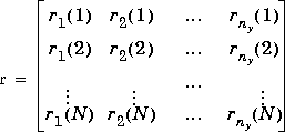
Is normally a setpoint matrix consisting of N rows and ny columns, where ny is the number of output variables, y:

where ri(k) is the setpoint for output j at time t = kT, and T is the sampling period (as specified in the step format of plant and model). If tend > NT, the setpoints vary for the first N periods in the simulation, as specified by r, and are then held constant at the values given in the last row of r for the remainder of the simulation.

In many simulations one wants the setpoints to be constant for the entire time, in which case r need only contain a single row of ny values.

    If you set r=[ ], the default is a row of ny zeros.

For open-loop simulations, r specifies the manipulated variables and must contain nu columns.

The following input variables are optional. In general, setting one of them equal to an empty matrix causes mpcsim to use the default value, which is given in the description.

usat
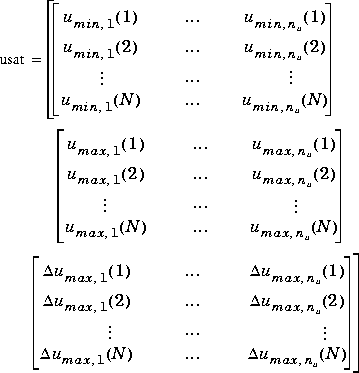
Is a matrix giving the limits on the manipulated variables. Its format is as follows:

Note that it contains three matrices of N rows. N may be different than that for the setpoint matrix, r, but the idea is the same: the saturation limits will vary for the first N sampling periods of the simulation, then be held constant at the values given in the last row of usat for the remaining periods (if any).

The first matrix specifies the lower bounds on the nu manipulated variables. For example, umin,j(k) is the lower bound for manipulated variable j at time t = kT in the simulation. If umin,j(k) = -inf, manipulated variable j will have no lower bound at t = kT.

The second matrix gives the upper bounds on the manipulated variables. If umax,j(k) = inf, manipulated variable j will have no upper bound at t = kT.

The lower and upper bounds may be either positive or negative (or zero) as long as umin,j(k) umax,j(k).

The third matrix gives the limits on the rate of change of the manipulated variables. In other words, mpcsim will force
|uj(k) - uj(k - 1)| umax,j(k). The limits on the rate of change must be nonnegative.

The default is no saturation constraints, i.e., all the umin values will be set to -inf, and all the umax and umax values will be set to inf.

Note: Saturation constraints in mpcsim are enforced by simply clipping the manipulated variable moves so that they satisfy all constraints. This is a nonoptimal solution that, in general, will differ from the results you would get using the ulim variable in cmpc.

tfilter
Is a matrix of time constants for the noise filter and the unmeasured disturbances entering at the plant output. The first row of ny elements gives the noise filter time constants and the second row of ny elements gives the time constants of the lags through which the unmeasured disturbance steps pass. If tfilter only contains one row, the unmeasured disturbances are assumed to be steps. If you set tfilter=[ ] or omit it, the default is no noise filtering and steplike unmeasured disturbances.

dplant
Is a model in MPC step format representing all the disturbances (measured and unmeasured) that affect plant in the above diagram. If dplant is provided, then input dstep is also required. For output step disturbances, set dplant=[ ]. The default is no disturbances.

dmodel
Is a model in MPC step format representing the measured disturbances. If dmodel is provided, then input dstep is also required. If there are no measured disturbances, set dmodel=[ ]. For output step disturbances, set dmodel=[ ]. If there are both measured and un- measured disturbances, set the columns of dmodel corresponding to the unmeasured disturbances to zero. The default is no measured disturbances.

dstep
Is a matrix of disturbances to the plant. For output step disturbances (dplant=[ ] and dmodel=[ ]), the format is the same as for r. For disturbances through step-response models (dplant only or both dplant and dmodel nonempty), the format is the same as for r, except that the number of columns is nd rather than ny. The default is a row of zeros.

Note: You may use a different number of rows in the matrices r, usat and dstep, should that be appropriate for your simulation.

The calculated outputs are as follows (all but yp are optional):

yp
Is a matrix containing M rows and ny columns, where M = round(tend/delt2) + 1 and delt2 is the sampling time. The first row will contain the initial condition, and row k - 1 will give the values of the plant outputs, y (see above diagram), at time t = kT.

u

Is a matrix containing the same number of rows as yp and nu columns. The time corresponding to each row is the same as for yp. The elements in each row are the values of the manipulated variables, u (see above diagram).

ym

Is a matrix of the same structure as yp, containing the values of the predicted outputs from the state estimator in the controller. ym will, in general, differ from yp if modelplant and/or there are unmeasured disturbances. The prediction includes the effect of the most recent measurement, i.e.,.

Examples
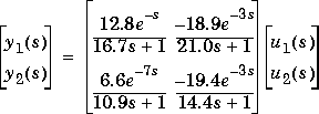
Consider the linear system:

The following statements build the model and calculate the MPC controller gain:

• g11=poly2tfd(12.8,[16.7 1],0,1);
  g21=poly2tfd(6.6,[10.9 1],0,7);
  g12=poly2tfd(-18.9,[21.0 1],0,3);
  g22=poly2tfd(-19.4,[14.4 1],0,3);
  delt=3; ny=2; tfinal=90; 
  model=tfd2step(tfinal,delt,ny,g11,g21,g12,g22); 
  plant=model; 
  P=6; M=2; 
  ywt=[ ]; uwt=[1 1]; 
  Kmpc=mpccon(imod,ywt,uwt,M,P);
  

• tend=30; r=[0 1]; 
  [y,u]=mpcsim(plant,model,Kmpc,tend,r); 
  plotall(y,u,delt),pause
  
  
  
  

• r=[ ]; usat=[ ]; tfilter=[ ]; dmodel=[ ]; 
  dplant=plant; 
  dstep=[ 1 0; 0 0]; 
  [y,u]=mpcsim(plant,model,Kmpc,tend,r,usat,tfilter,...
      dplant,dmodel,dstep); 
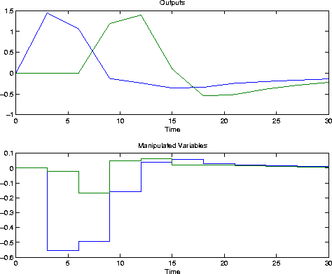
  plotall(y,u,delt),pause
  
  
  
  

• usat=[-inf -inf inf inf 0.1 0.05];
  [y,u]=mpcsim(plant,model,Kmpc,tend,r,usat,tfilter,... 
      dplant,dmodel,dstep); 
  plotall(y,u,delt),pause
  
  
  

Restriction
Initial conditions of zero are used for all the variables. This simulates the condition where all variables represent a deviation from a steady-state initial condition.

See Also
plotall, ploteach, cmpc, mpccl, mpccon

mpcinfo

nlcmpc