Fitting Data (Curve Fitting Toolbox)

Curve Fitting Toolbox

Example: Fitting with Custom Equations

You can define your own equations with the Create Custom Equation GUI. You open this GUI one of two ways:

From the Curve Fitting Tool, select Tools->Custom Equation.
From the Fitting GUI, select Custom Equations from the Type of fit list, then click the New Equation button.

The Create Custom Equation GUI contains two panes: one for creating linear custom equations and one for creating general (nonlinear) custom equations. These panes are described in the following examples.

Linear Equation: Legendre Polynomial Fit

This example fits data using several custom linear equations. The data is generated, and is based on the nuclear reaction ¹²C(e,e')⁸Be. The equations use sums of Legendre polynomial terms.

Consider an experiment in which 124 MeV electrons are scattered from ¹²C nuclei. In the subsequent reaction, alpha particles are emitted and produce the residual nuclei ⁸Be. By analyzing the number of alpha particles emitted as a function of angle, you can deduce certain information regarding the nuclear dynamics of ¹²C. The reaction kinematics are shown below.

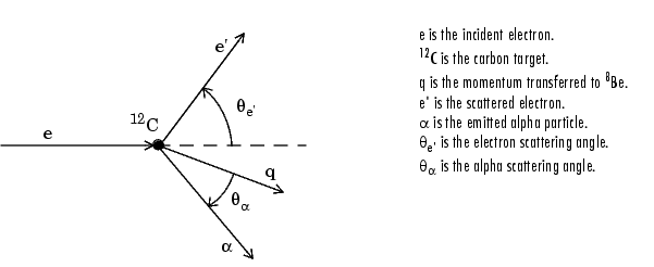
The data is collected by placing solid state detectors at values of ranging from 10^o to 240^o in 10^o increments.

It is sometimes useful to describe a variable expressed as a function of angle in terms of Legendre polynomials

where P_n(x) is a Legendre polynomial of degree n, x is cos(), and a_n are the coefficients of the fit. Refer to MATLAB's legendre function for information about generating Legendre polynomials.

For the alpha-emission data, you can directly associate the coefficients with the nuclear dynamics by invoking a theoretical model, which is described in [8]. Additionally, the theoretical model introduces constraints for the infinite sum shown above. In particular, by considering the angular momentum of the reaction, a fourth-degree Legendre polynomial using only even terms should describe the data effectively.

You can generate Legendre polynomials with Rodrigues' formula:

The Legendre polynomials up to fourth degree are given below.

Table 3-4: Legendre Polynomials up to Fourth Degree
n
P_n(x)

0
1

1
x

2
(1/2)(3x²- 1)

3
(1/2)(5x³ - 3x)

4
(1/8)(35x⁴ - 30x² + 3)

**Table 3-4: Legendre Polynomials up to Fourth Degree**
n	P_n(x)
0	1
1	x
2	(1/2)(3x²- 1)
3	(1/2)(5x³ - 3x)
4	(1/8)(35x⁴ - 30x² + 3)

The first step is to load the ¹²C alpha-emission data from the file carbon12alpha.mat, which is provided with the toolbox.

```
load carbon12alpha
```

The workspace now contains two new variables, angle and counts:

angle is a vector of angles (in radians) ranging from 10^o to 240^o in 10^o increments.
counts is a vector of raw alpha particle counts that correspond to the emission angles in angle.

Import these two variables into the Curve Fitting Toolbox and name the data set C12Alpha.

The Fit Editor for a custom equation fit type is shown below.

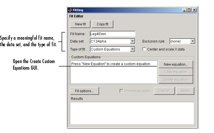
Fit the data using a fourth-degree Legendre polynomial with only even terms:

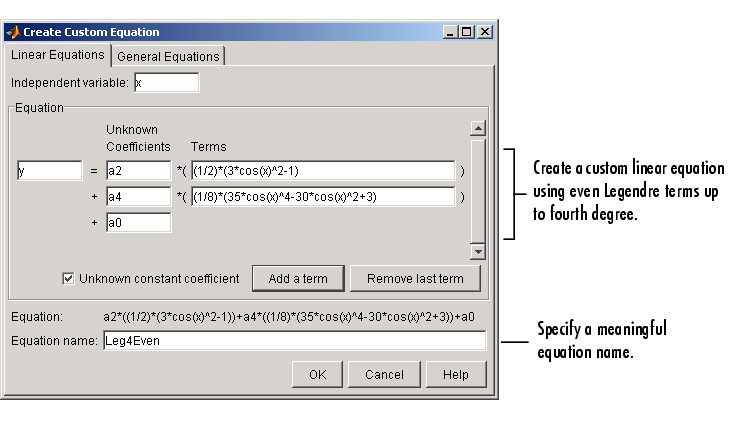
Because the Legendre polynomials depend only on the predictor variable and constants, you use the Linear Equations pane on the Create Custom Equation GUI. This pane is shown below for the model given by y₁(x). Note that because angle is given in radians, the argument of the Legendre terms is given by cos().

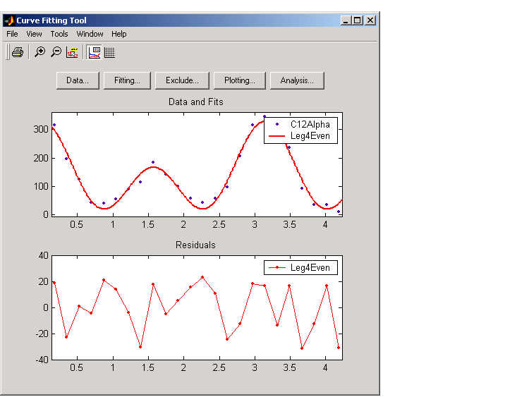
The fit and residuals are shown below. The fit appears to follow the trend of the data well, while the residuals appear to be randomly distributed and do not exhibit any systematic behavior.

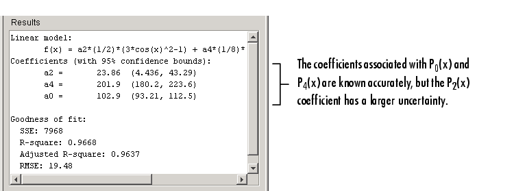
The numerical fit results are shown below. The 95% confidence bounds indicate that the coefficients associated with P₀(x) and P₄(x) are known fairly accurately, but that the P₂(x) coefficient has a relatively large uncertainty.

To confirm the theoretical argument that the alpha-emission data is best described by a fourth-degree Legendre polynomial with only even terms, fit the data using both even and odd terms:

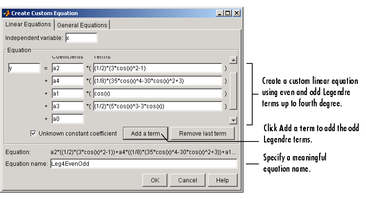
The Linear Equations pane of the Create Custom Equation GUI is shown below for the model given by y₂(x).

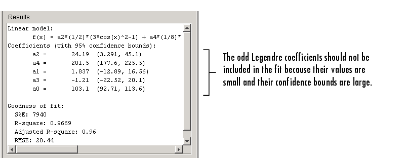
The numerical results indicate that the odd Legendre terms do not contribute significantly to the fit, and the even Legendre terms are essentially unchanged from the previous fit. This confirms that the initial model choice is the best one.

General Equation: Fourier Series Fit

This example fits the ENSO data using several custom nonlinear equations. The ENSO data consists of monthly averaged atmospheric pressure differences between Easter Island and Darwin, Australia. This difference drives the trade winds in the southern hemisphere.

As shown in Example: Smoothing Data, the ENSO data is clearly periodic, which suggests it can be described by a Fourier series

where a_i and b_i are the amplitudes, and c_i are the periods (cycles) of the data. The question to be answered in this example is how many cycles exist? As a first attempt, assume a 12 month cycle and fit the data using one sine term and one cosine term.

If the fit does not describe the data well, add additional sine and cosine terms with unique period coefficients until a good fit is obtained.

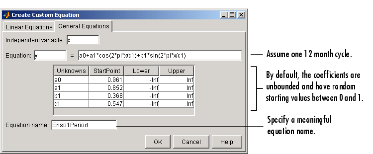
Because there is an unknown coefficient c₁ included as part of the trigonometric function arguments, the equation is nonlinear. Therefore, you must specify the equation using the General Equations pane of the Create Custom Equation GUI. This pane is shown below for the equation given by y₁(x).

Note that the toolbox includes the Fourier series as a nonlinear library equation. However, the library equation does not meet the needs of this example because its terms are defined as fixed multiples of the fundamental frequency w. Refer to Fourier Series for more information.

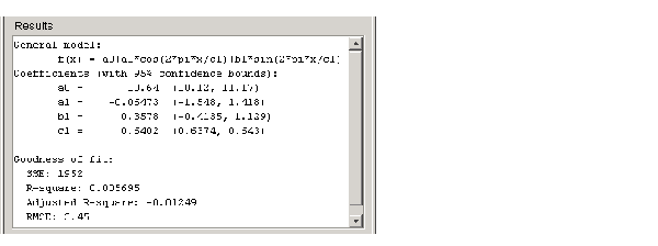
The numerical results shown below indicate that the fit does not describe the data well. In particular, the fitted value for c1 is unreasonably small. Because the starting points are randomly selected, your initial fit results might differ from the results shown here.

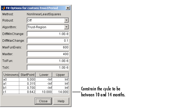
To assist the fitting procedure, constrain c1 to a value between 10 and 14. To define constraints for unknown coefficients, use the Fit Options GUI, which you open by clicking the Fit options button in the Fitting GUI.

The fit, residuals, and numerical results are shown below.

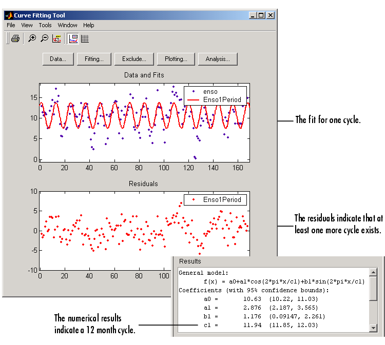
The fit appears to be reasonable for some of the data points but clearly does not describe the entire data set very well. As predicted, the numerical results indicate a cycle of approximately 12 months. However, the residuals show a systematic periodic distribution indicating that there are additional cycles that you should include in the fit equation. Therefore, as a second attempt, add an additional sine and cosine term to y₁(x)

and constrain the upper and lower bounds of c₂ to be roughly twice the bounds used for c₁.

The fit, residuals, and numerical results are shown below.

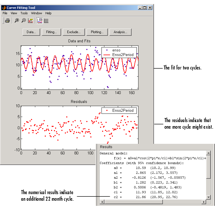
The fit appears to be reasonable for most of the data points. However, the residuals indicate that you should include another cycle to the fit equation. Therefore, as a third attempt, add an additional sine and cosine term to y₂(x)

and constrain the lower bound of c₃ to be roughly three times the value of c₁.

The fit, residuals, and numerical results are shown below.

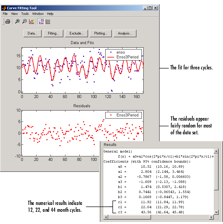
The fit is an improvement over the previous two fits, and appears to account for most of the cycles present in the ENSO data set. The residuals appear random for most of the data, although a pattern is still visible indicating that additional cycles may be present, or you can improve the fitted amplitudes.

In conclusion, Fourier analysis of the data reveals three significant cycles. The annual cycle is the strongest, but cycles with periods of approximately 44 and 22 months are also present. These cycles correspond to El Nino and the Southern Oscillation (ENSO).

General Equation: Gaussian Fit with Exponential Background

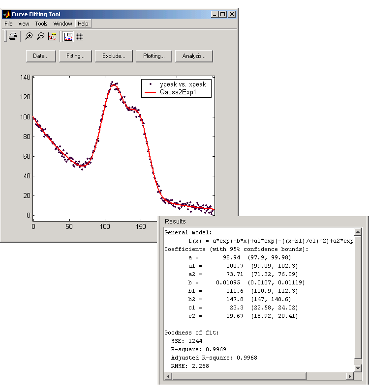
This example fits two poorly resolved Gaussian peaks on a decaying exponential background using a general (nonlinear) custom model. To get started, load the data from the file gauss3.mat, which is provided with the toolbox.

```
load gauss3
```

The workspace now contains two new variables, xpeak and ypeak:

xpeak is a vector of predictor values.
ypeak is a vector of response values.

Import these two variables into the Curve Fitting Toolbox and accept the default data set name ypeak vs. xpeak.

You will fit the data with the following equation

where a_i are the peak amplitudes, b_i are the peak centroids, and c_i are related to the peak widths. Because there are unknown coefficients included as part of the exponential function arguments, the equation is nonlinear. Therefore, you must specify the equation using the General Equations pane of the Create Custom Equation GUI. This pane is shown below for y(x).

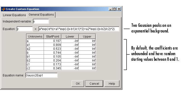
The data, fit, and numerical fit results are shown below. Clearly, the fit is poor.

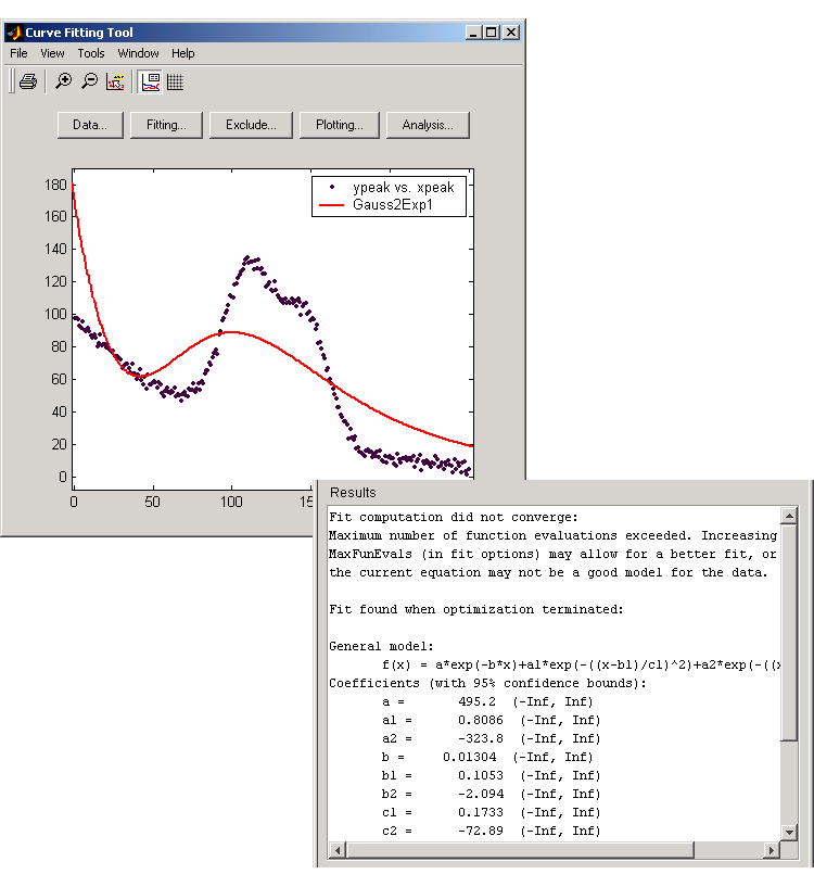
Because the starting points are randomly selected, your initial fit results might differ from the results shown here.

The results include this warning message.

Fit computation did not converge:
Maximum number of function evaluations exceeded. Increasing
MaxFunEvals (in fit options) may allow for a better fit, or 
the current equation may not be a good model for the data.

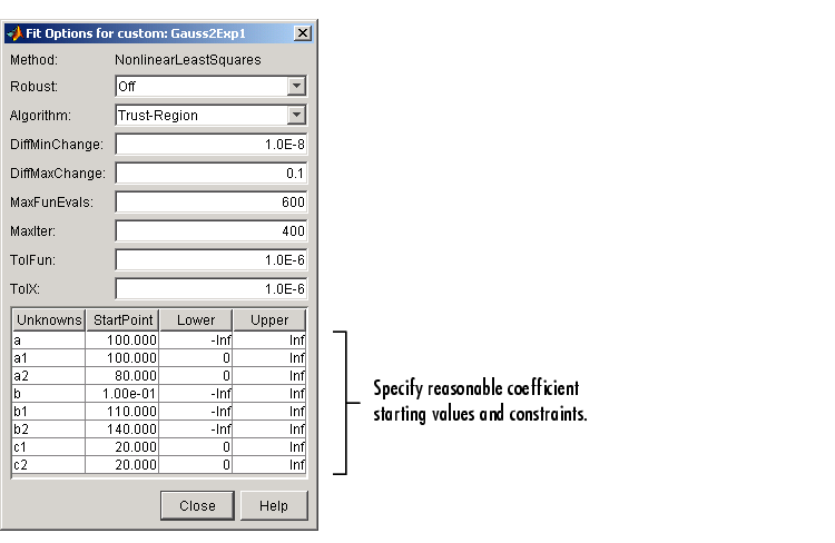
To improve the fit for this example, specify reasonable starting points for the coefficients. Deducing the starting points is particularly easy for the current model because the Gaussian coefficients have a straightforward interpretation and the exponential background is well defined. Additionally, as the peak amplitudes and widths cannot be negative, constrain a₁, a₂, c₁, and c₂ to be greater then zero.

To define starting values and constraints for unknown coefficients, use the Fit Options GUI, which you open by clicking the Fit options button. The starting values and constraints are shown below.

The data, fit, residuals, and numerical results are shown below.

Example: Rational Fit Example: Robust Fit