

| Curve Fitting Toolbox |   |
Example: Rational Fit
This example fits measured data using a rational model. The data describes the coefficient of thermal expansion for copper as a function of temperature in degrees Kelvin.
To get started, load the thermal expansion data from the file hahn1.mat, which is provided with the toolbox.
The workspace now contains two new variables, temp and thermex:
temp is a vector of temperatures in degrees Kelvin.
thermex is a vector of thermal expansion coefficients for copper.
Import these two variables into the Curve Fitting Tool and name the data set CuThermEx.
For this data set, you will find the rational equation that produces the best fit. As described in Library Models, rational models are defined as a ratio of polynomials

where n is the degree of the numerator polynomial and m is the degree of the denominator polynomial. Note that the rational equations are not associated with physical parameters of the data. Instead, they provide a simple and flexible empirical model that you can use for interpolation and extrapolation.
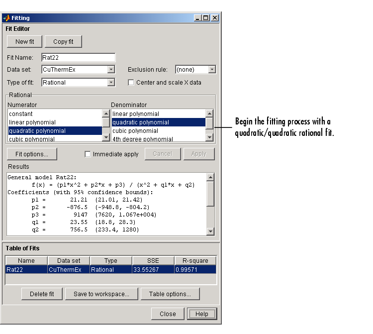
As you can see by examining the shape of the data, a reasonable initial choice for the rational model is quadratic/quadratic. The Fitting GUI configured for this equation is shown below.
The data, fit, and residuals are shown below.
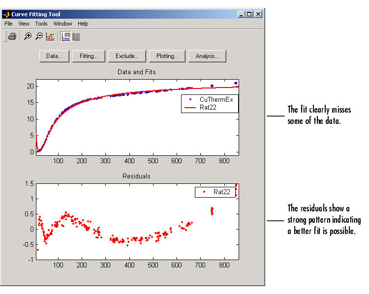
The fit clearly misses the data for the smallest and largest predictor values. Additionally, the residuals show a strong pattern throughout the entire data set indicating that a better fit is possible.
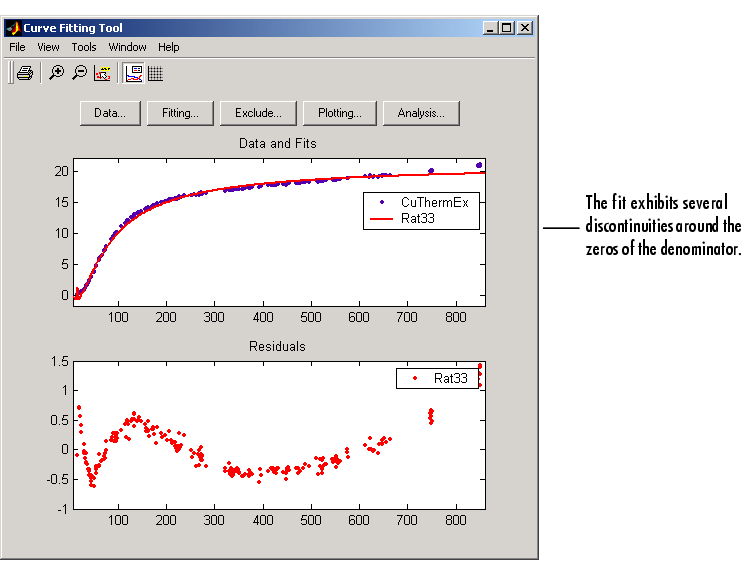
For the next fit, try a cubic/cubic equation. The data, fit, and residuals are shown below.
The numerical results shown below indicate that the fit did not converge.
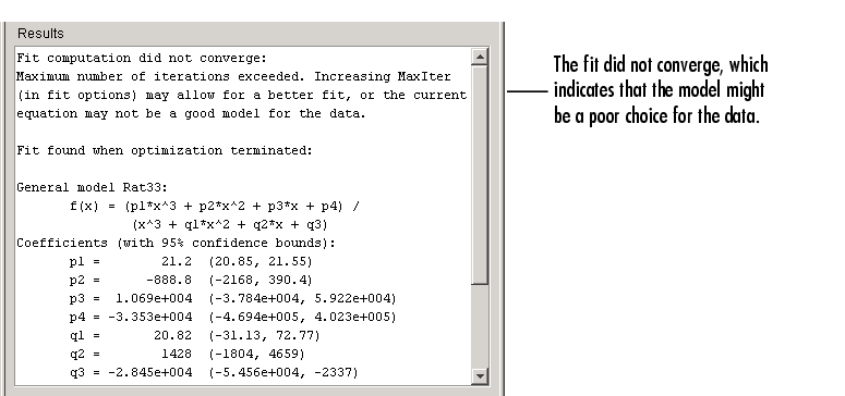
Although the message in the Results window indicates that you might improve the fit if you increase the maximum number of iterations, a better choice at this stage of the fitting process is to use a different rational equation because the current fit contains several discontinuities. These discontinuities are due to the function blowing up at predictor values that correspond to the zeros of the denominator.
As the next try, fit the data using a cubic/quadratic equation. The data, fit, and residuals are shown below.
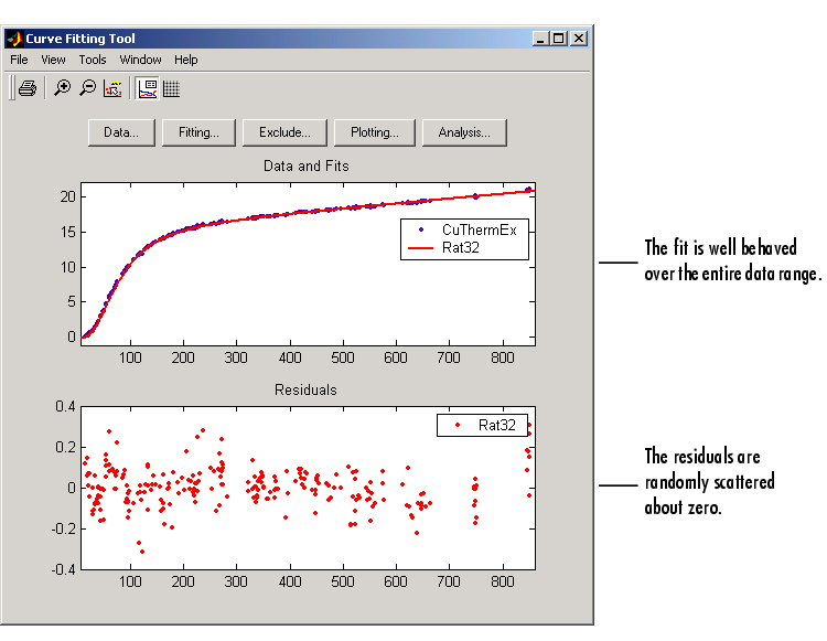
The fit is well behaved over the entire data range, and the residuals are randomly scattered about zero. Therefore, you can confidently use this fit for further analysis.
 | Evaluating the Goodness of Fit | Example: Fitting with Custom Equations |  |