

| Curve Fitting Toolbox | |
Example: Robust Fit
This example fits data that is assumed to contain one outlier. The data consists of the 2000 United States presidential election results for the state of Florida. The fit model is a first degree polynomial and the fit method is robust linear least squares with bisquare weights.
In the 2000 presidential election, many residents of Palm Beach County, Florida, complained that the design of the election ballot was confusing, which they claim led them to vote for the Reform candidate Pat Buchanan instead of the Democratic candidate Al Gore. The so-called "butterfly ballot" was used only in Palm Beach County and only for the election-day ballots for the presidential race. As you will see, the number of Buchanan votes for Palm Beach is far removed from the bulk of data, which suggests that the data point should be treated as an outlier.
To get started, load the Florida election result data from the file flvote2k.mat, which is provided with the toolbox.
The workspace now contains these three new variables:
buchanan is a vector of votes for the Reform Party candidate Pat Buchanan.
bush is a vector of votes for the Republican Party candidate George Bush.
gore is a vector of votes for the Democratic Party candidate Al Gore.
Each variable contains 68 elements, which correspond to the 67 Florida counties plus the absentee ballots. The names of the counties are given in the variable counties. From these variables, create two data sets with the Buchanan votes as the response data: buchanan vs. bush and buchanan vs. gore.
For this example, assume that the relationship between the response and predictor data is linear with an offset of zero.
m1 is the number of Bush votes expected for each Buchanan vote, and m2 is the number of Gore votes expected for each Buchanan vote.
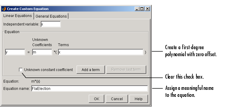
To create a first-degree polynomial equation with zero offset, you must create a custom linear equation. As described in Example: Fitting with Custom Equations, you can create a custom equation using the Fitting GUI by selecting Custom Equations from the Type of fit list, and then clicking the New Equation button.
The Linear Equations pane of the Create Custom Equation GUI is shown below.
Before fitting, you should exclude the data point associated with the absentee ballots from each data set because these voters did not use the butterfly ballot. As described in Marking Outliers, you can exclude individual data points from a fit either graphically or numerically using the Exclude GUI. For this example, you should exclude the data numerically. The index of the absentee ballot data is given by
The Exclude GUI is shown below.
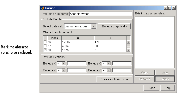
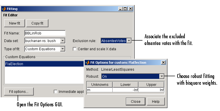
The exclusion rule is named AbsenteeVotes. You use the Fitting GUI to associate an exclusion rule with the data set to be fit.
For each data set, perform a robust fit with bisquare weights using the FlaElection equation defined above. For comparison purposes, also perform a regular linear least squares fit. Refer to Robust Least Squares for a description of the robust fitting methods provided by the toolbox.
You can identify the Palm Beach County data in the scatter plot by using the data tips feature, and knowing the index number of the data point.
The Fit Editor and the Fit Options GUI are shown below for a robust fit.
The data, robust and regular least squares fits, and residuals for the buchanan vs. bush data set are shown below.
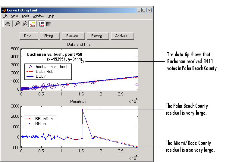
The graphical results show that the linear model is reasonable for the majority of data points, and the residuals appear to be randomly scattered around zero. However, two residuals stand out. The largest residual corresponds to Palm Beach County. The other residual is at the largest predictor value, and corresponds to Miami/Dade County.
The numerical results are shown below. The inverse slope of the robust fit indicates that Buchanan should receive one vote for every 197.4 Bush votes.
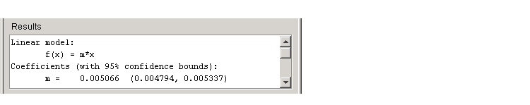
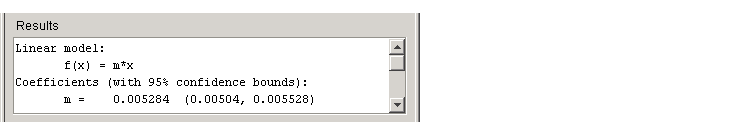
The data, robust and regular least squares fits, and residuals for the buchanan vs. gore data set are shown below.
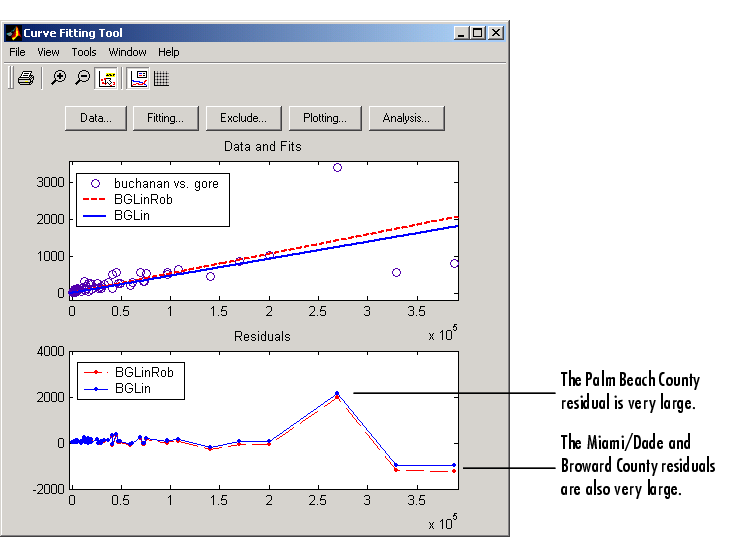
Again, the graphical results show that the linear model is reasonable for the majority of data points, and the residuals appear to be randomly scattered around zero. However, three residuals stand out. The largest residual corresponds to Palm Beach County. The other residuals are at the two largest predictor values, and correspond to Miami/Dade County and Broward County.
The numerical results are shown below. The inverse slope of the robust fit indicates that Buchanan should receive one vote for every 189.3 Gore votes.
Using the fitted slope value, you can determine the expected number of votes that Buchanan should have received for each fit. For the Buchanan versus Bush data, you evaluate the fit at a predictor value of 152,951. For the Buchanan versus Gore data, you evaluate the fit at a predictor value of 269,732. These results are shown below for both data sets and both fits.
The robust results for the Buchanan versus Bush data suggest that Buchanan received 3411 - 775 = 2636 excess votes, while robust results for the Buchanan versus Gore data suggest that Buchanan received 3411 - 1425 = 1986 excess votes.
The margin of victory for George Bush is given by
Therefore, the voter intention comes into play because in both cases, the margin of victory is less than the excess Buchanan votes.
In conclusion, the analysis of the 2000 United States presidential election results for the state of Florida suggests that the Reform Party candidate received an excess number of votes in Palm Beach County, and that this excess number was a crucial factor in determining the election outcome. However, additional analysis is required before a final conclusion can be made.
| | Example: Fitting with Custom Equations | Nonparametric Fitting | |