sfl, sfr (Robust Control Toolbox)

Robust Control Toolbox

sfl, sfr

Left and right spectral factorization.

Syntax

[am,bm,cm,dm] = sfl(a,b,c,d)
[am,bm,cm,dm] = sfr(a,b,c,d) 
[ssm] = sfl(ss)
[ssm] = sfr(ss)

Description
Given a stabilizable realization of a transfer function G(s) := (A, B, C, D) with , sfl computes a left spectral factor M(s) such that

where M(s) := (A_M, B_M, C_M, D_M) is outer (i.e., stable and minimum-phase).

Sfr computes a right spectral factor M(s) of G(s) such that

Algorithm
Given a transfer function G(s) := (A, B, C, D), the LQR optimal control
u = -Fx = -R^-1(XB + N)^Tx stabilizes the system and minimize the quadratic cost function

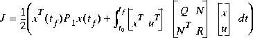
as 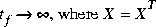satisfies the algebraic Riccati equation

Moreover, the optimal return difference I + L(s) = I + F(Is - A) ^-1B satisfies the optimal LQ return difference equality:

where (s) = (Is - A)^-1B, and *(s) = ^T(-s). Taking

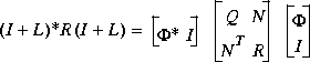
the return difference equality reduces to

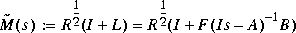
so that a minimum phase, but not necessarily stable, spectral factor is

where X and F can simply be obtained by the command:

[F,X] = lqr(A,B,Q,R,N) =
lqr(A,B,-C'*C,(I-D'*D),-C'*D).

Finally, to get the stable spectral factor, we take M(s) to be the inverse of the

outer factor of . The routine iofr is used to compute the outer factor.

Limitations
The spectral factorization algorithm employed in sfl and sfr requires the system G(s) to have and to have no -axis poles. If the condition fails to hold, the Riccati subroutine (aresolv) will normally produce the message

WARNING: THERE ARE j-AXIS POLES... 
RESULTS MAY BE INCORRECT !!

This happens because the Hamiltonian matrix associated with the LQR optimal control problem has j

-axis eigenvalues if and only if

. An interesting implication is that you could use sfl or sfr to check whether

without the need to actually compute the singular value Bode plot of G(j

See Also
iofc, iofr

sectf ssv