| Robust Control Toolbox | |
Continuous characteristic gain loci frequency response.
Discrete characteristic gain loci frequency response.
Syntax
[cg,ph,w] = (d)cgloci(a,b,c,d(,Ts)) [cg,ph,w] = (d)cgloci(a,b,c,d(,Ts),'inv') [cg,ph,w] = (d)cgloci(a,b,c,d(,Ts),w) [cg,ph,w] = (d)cgloci(a,b,c,d(,Ts),w,'inv')[cg,ph,w] = (d)cgloci(ss,)
Description
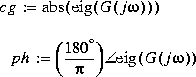
cgloci computes the matrices cg and ph containing the characteristic gain and phase of the frequency response matrix 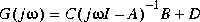 as a function of frequency,
  . The characteristic gain
 cg and phase ph vectors are defined as
When invoked without lefthand arguments, cgloci produces a characteristic gain and phase Bode plot on the screen. The frequency range is chosen automatically and incorporates more points where the plot is changing rapidly.
cgloci(a,b,c,d,'inv') plots the characteristic gain and phase loci of the inverse system G(s)-1.
When the frequency vector w is supplied, the vector w specifies the frequencies in radians/sec at which the char. loci will be computed. See logspace to generate frequency vectors that are equally spaced logarithmically in frequency.
When invoked with lefthand arguments,
returns the gain, phase matrices and the frequency point in the vectorw.
dcgloci computes the discrete version of the characteristic loci by replacing
G(j) by  . The variable
 Ts is the sampling period.
Cautionary Note
Nyquist loci and Bode plots of characteristic gain loci can produce a misleadingly optimistic picture of the stability margins multiloop systems. For this reason, it is usually a good idea when using cgloci to also examine the singular value Bode plots in assessing stability robustness. See sigma and dsigma.
Examples
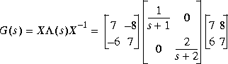
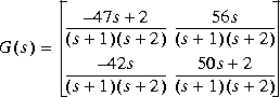
Let's consider a 2 by 2 transfer function matrix of the plant [1]
The controller is a diagonal constant gain matrix
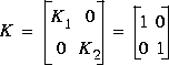
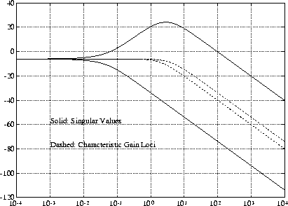
The characteristic gain loci containing in  (s) seem to imply that the system has infinity gain margin and ± 180 degree phase margin in each of the feedback loop. However, if you slightly perturb the gains K1 and K2 to K1 + 0.13 and
K2 - 0.12 simultaneously, the system becomes unstable!
On the other hand, the singular value Bode plot of the complementary sensitivity 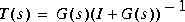 (MATLAB command:
 sigma) easily predicts the system robustness (see Tutorial). See Figure 1-4.
The resonance peak of the maximum singular value ( 16.2695) predicts that
the multiplicative uncertainty can only be as large as
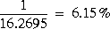
before instability occurs.
Figure 1-4: Singular Value vs. Characteristic Gain Loci.
Alternatively, you can compute guaranteed stability margins using the formulae given in Singular-Value Loop-Sharing: The Mixed-Sensitivity Approach [2]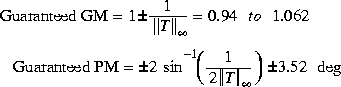
which clearly predict the poor robustness of the system. These guaranteed stability margins provide a tolerance such that you can vary both gain and phase simultaneously in all the feedback loops.
See Also
bode, dsigma, dbode, logspace, sigma
[1] J. C. Doyle, "Robustness of Multiloop Linear Feedback Systems," Proc. IEEE Conf. on Decision and Control, San Diego, CA, Jan. 10-12, 1979
[2] N. A. Lehtomaki, N. R. Sandell, Jr., and M. Athans, "Robustness Results in Linear-Quadratic Gaussian Based Multivariable Control Designs," IEEE Trans. on Automat. Contr., vol. AC-26, No. 1, pp. 75-92, Feb. 1981.
[3] I. Postlethwaite and A. G. J. MacFarlane, A Complex Variable Approach to the Analysis of Linear Multivariable Feedback Systems, Springer-Verlag, 1979.
| bstschml, bstschmr | daresolv | |