Examples (Partial Differential Equation Toolbox)

Partial Differential Equation Toolbox

Examples of Parabolic Problems

This section describes the solution of some parabolic PDE problems. The problems are solved using both the graphical user interface and the command-line functions of the PDE Toolbox. The topics include

The Heat Equation: A Heated Metal Block

A common parabolic problem is the heat equation:

The heat equation describes the diffusion of heat in a body of some kind. See the section Application Modes for more information about heat transfer and diffusion problems.

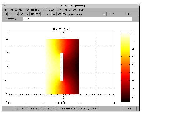
This first example studies a heated metal block with a rectangular crack or cavity. The left side of the block is heated to 100 degrees centigrade. At the right side of the metal block, heat is flowing from the block to the surrounding air at a constant rate. All the other block boundaries are isolated. This leads to the following set of boundary conditions (when proper scaling of t is chosen):

on the left side (Dirichlet condition)
on the right side (Neumann condition)
on all other boundaries (Neumann condition)

Also, for the heat equation we need an initial value: the temperature in the metal block at the starting time t₀. In this case, the temperature of the block is 0 degrees at the time we start applying heat.

Finally, to complete the problem formulation, we specify that the starting time is 0 and that we want to study the heat distribution during the first five seconds.

Using the Graphical User Interface

Once you have started the pdetool GUI and selected the Generic Scalar mode, drawing the CSG model can be done very quickly: Draw a rectangle (R1) with the corners in x = [-0.5 0.5 0.5 -0.5] and y = [-0.8 -0.8 0.8 0.8]. Draw another rectangle (R2) to represent the rectangular cavity. Its corners should have the coordinates x = [-0.05 0.05 0.05 -0.05] and y = [-0.4 -0.4 0.4 0.4]. To assist in drawing the narrow rectangle representing the cavity, open the Grid Spacing dialog box from the Options and enter x-axis extra ticks at -0.05 and 0.05. Then turn on the grid and the "snap-to-grid" feature. A rectangular cavity with the correct dimensions is then easy to draw.

The CSG model of the metal block is now simply expressed as the set formula R1-R2.

Leave the Draw mode and enter the Boundary mode by clicking the button, and continue by selecting boundaries and specifying the boundary conditions. Using the Select All option from the Edit menu and then defining the Neumann condition

for all boundaries first is a good idea since that leaves only the leftmost and rightmost boundaries to define individually.

The next step is to open the PDE Specification dialog box and enter the PDE coefficients.

The generic parabolic PDE that the PDE Toolbox solves is

with initial values u0 = u(t₀) and the times at which to compute a solution specified in the array tlist.

For this case, you have d = 1, c = 1, a = 0, and f = 0.

Initialize the mesh by clicking the button. If you want, you can refine the mesh by clicking the Refine button.

The initial values u0 = 0, and the list of times is entered as the MATLAB array [0:0.5:5]. They are entered into the Solve Parameters dialog box, which is accessed by selecting Parameters . . . from the Solve menu.

The problem can now be solved. Pressing the = button solves the heat equation at 11 different times from 0 to 5 seconds. By default, an interpolated plot of the solution, i.e., the heat distribution, at the end of the time span is displayed.

A more interesting way to visualize the dynamics of the heat distribution process is to animate the solution. To start an animation, check the Animation check box in the Plot selection dialog box. Also, select the colormap hot. Click the Plot button to start a recording of the solution plots in a separate figure window. The recorded animation is then "played" five times.

Note that the temperature in the block rises very quickly. To improve the animation and focus on the first second, try to change the list of times to the MATLAB expression logspace(-2,0.5,20).

Also, try to change the heat capacity coefficient d and the heat flow at the rightmost boundary to see how they affect the heat distribution.

Using Command-Line Functions

First, you must create geometry and boundary condition M-files. The M-files used here were created using pdetool. The geometry of the metal block is described in crackg.m, and the boundary conditions can be found in crackb.m.

To create an initial mesh, call initmesh:

```
» [p,e,t]=initmesh('crackg'); 
```

The heat equation can now be solved using the PDE Toolbox function parabolic. The generic parabolic PDE that parabolic solves is

with initial value u0 = u(t₀) and the times at which to compute a solution specified in the array tlist. For this case, you have d = 1, c = 1, a = 0, and f = 0. The initial value u0 = 0, and the list of times, tlist, is set to the MATLAB array 0:0.5:5.

To compute the solution, call parabolic:

 u=parabolic(0,0:0.5:5,'crackb',p,e,t,1,0,0,1);

The solution u created this way a matrix with 11 columns, where each column corresponds to the solution at the 11 points in time 0,0.5, . . . ,4.5,5.0.

Let us plot the solution at t = 5.0 seconds using interpolated shading and a hidden mesh. Use the hot colormap:

 pdeplot(p,e,t,'xydata',u(:,11),'mesh','off',...
'colormap','hot')

Domain Decomposition Heat Distribution in Radioactive Rod