Partial Differential Equation Toolbox

Domain Decomposition

The PDE Toolbox is designed to deal with one-level domain decomposition. If has a complicated geometry, it is often useful to decompose it into the union of more subdomains of simpler structure. Such structures are often introduced by pdetool.

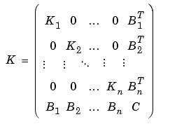
Assume now that is the disjoint union of some subdomains ₁, ₂, . . . , n. Then you could renumber the nodes of a mesh on such that the indices of the nodes of each subdomain are grouped together, while all the indices of nodes common to two or more subdomains come last. Since K has nonzero entries only at the lines and columns that are indices of neighboring nodes, the stiffness matrix is partitioned as follows:

while the right side is

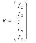
The PDE Toolbox routine assempde can assemble the matrices Kj, Bj, fj, and C separately. You have full control over the storage and further processing of these matrices.

Furthermore, the structure of the linear system

Ku = F

is simplified by decomposing K into the partitioned matrix above.

Now consider the geometry of the L-shaped membrane. You can plot the geometry of the membrane by typing

• pdegplot('lshapeg')
  

Notice the borders between the subdomains. There are three subdomains. Thus the matrix formulas with n = 3 from above can be used. Now generate a mesh for the geometry:

• [p,e,t]=initmesh('lshapeg'); 
  [p,e,t]=refinemesh('lshapeg',p,e,t); 
  [p,e,t]=refinemesh('lshapeg',p,e,t); 
  

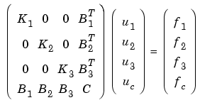
So for this case, with n = 3, you have

and the solution is given by block elimination:

In the MATLAB solution below, a more efficient algorithm using Choleski factorization is used:

• time=[]; 
  np=size(p,2); 
  % Find common points 
  c=pdesdp(p,e,t); 
  
  nc=length(c); 
  C=zeros(nc,nc); 
  FC=zeros(nc,1); 
  
  [i1,c1]=pdesdp(p,e,t,1);ic1=pdesubix(c,c1); 
  [K,F]=assempde('lshapeb',p,e,t,1,0,1,time,1); 
  K1=K(i1,i1);d=symmmd(K1);i1=i1(d); 
  K1=chol(K1(d,d));B1=K(c1,i1);a1=B1/K1; 
  C(ic1,ic1)=C(ic1,ic1)+K(c1,c1)-a1*a1'; 
  f1=F(i1);e1=K1'\f1;FC(ic1)=FC(ic1)+F(c1)-a1*e1; 
  
  [i2,c2]=pdesdp(p,e,t,2);ic2=pdesubix(c,c2); 
  [K,F]=assempde('lshapeb',p,e,t,1,0,1,time,2); 
  K2=K(i2,i2);d=symmmd(K2);i2=i2(d); 
  K2=chol(K2(d,d));B2=K(c2,i2);a2=B2/K2; 
  C(ic2,ic2)=C(ic2,ic2)+K(c2,c2)-a2*a2'; 
  f2=F(i2);e2=K2'\f2;FC(ic2)=FC(ic2)+F(c2)-a2*e2; 
  
  [i3,c3]=pdesdp(p,e,t,3);ic3=pdesubix(c,c3); 
  [K,F]=assempde('lshapeb',p,e,t,1,0,1,time,3); 
  K3=K(i3,i3);d=symmmd(K3);i3=i3(d); 
  K3=chol(K3(d,d));B3=K(c3,i3);a3=B3/K3; 
  C(ic3,ic3)=C(ic3,ic3)+K(c3,c3)-a3*a3'; 
  f3=F(i3);e3=K3'\f3;FC(ic3)=FC(ic3)+F(c3)-a3*e3; 
  
  % Solve 
  u=zeros(np,1); 
  u(c)=C\ FC; 
  u(i1)=K1\(e1-a1'*u(c1)); 
  u(i2)=K2\(e2-a2'*u(c2)); 
  u(i3)=K3\(e3-a3'*u(c3));
  

The problem can also be solved by typing

• % Compare with solution not using subdomains 
  [K,F]=assempde('lshapeb',p,e,t,1,0,1);u1=K\F; 
  norm(u-u1,'inf')
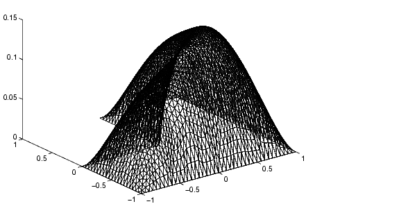
  pdesurf(p,t,u)
  

You can run this entire example by typing pdedemo4.

A Minimal Surface Problem

Examples of Parabolic Problems