Partial Differential Equation Toolbox

Heat Distribution in Radioactive Rod

This heat distribution problem is an example of a 3-D parabolic PDE problem that is reduced to a 2-D problem by using cylindrical coordinates.

Consider a cylindrical radioactive rod. At the left end, heat is continuously added. The right end is kept at a constant temperature. At the outer boundary, heat is exchanged with the surroundings by transfer. At the same time, heat is uniformly produced in the whole rod due to radioactive processes. Assume that the initial temperature is zero. This leads to the following problem:

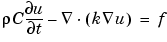
where is the density, C is the rod's thermal capacity, k is the thermal conductivity, and f is the radioactive heat source.

The density for this metal rod is 7800 kg/m³, the thermal capacity is
500 Ws/kgºC, and the thermal conductivity is 40 W/mºC. The heat source is 20000 W/m³. The temperature at the right end is 100 ºC. The surrounding temperature at the outer boundary is 100 ºC, and the heat transfer coefficient is 50 W/m²ºC. The heat flux at the left end is 5000 W/m².

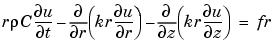
But this is a cylindrical problem, so you need to transform the equation, using the cylindrical coordinates r, z, and . Due to symmetry, the solution is independent of , so the transformed equation is

The boundary conditions are

• = 5000 at the left end of the rod (Neumann condition). Since the generalized Neumann condition in the PDE Toolbox is + qu = g, and c depends on r in this problem (c = kr), this boundary condition is expressed as = 5000r
• u = 100 at the right end of the rod (Dirichlet condition).
• = 50(100-u) at the outer boundary (generalized Neumann condition). In the PDE toolbox this must be expressed as
  + 50r · u = 50r · 100.
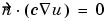• The cylinder axis r = 0 is not a boundary in the original problem, but in our 2-D treatment it has become one. We must give the artificial boundary condition here.

The initial value is u(t₀) = 0.

Using the Graphical User Interface

Solve this problem using the pdetool GUI. Model the rod as a rectangle with its base along the x-axis, and let the x-axis be the z direction and the y-axis be the r direction. A rectangle with corners in (-1.5,0), (1.5,0), (1.5,0.2), and (-1.5,0.2) would then model a rod with length 3 and radius 0.2.

Enter the boundary conditions by double-clicking the boundaries to open the Boundary Condition dialog box. For the left end, use Neumann conditions with 0 for q and 5000*y for g. For the right end, use Dirichlet conditions with 1 for h and 100 for r. For the outer boundary, use Neumann conditions with 50*y for q and 50*y*100 for g. For the axis, use Neumann conditions with 0 for q
and g.

Enter the coefficients into the PDE Specification dialog box: c is 40*y, a is zero, d is 7800*500*y, and f is 20000*y.

Animate the solution over a span of 20000 seconds (computing the solution every 1000 seconds). We can see how heat flows in over the right and outer boundaries as long as u < 100, and out when u > 100. You can also open the PDE Specification dialog box, and change the PDE type to Elliptic. This shows the solution when u does not depend on time, i.e., the steady state solution. The profound effect of cooling on the outer boundary can be demonstrated by setting the heat transfer coefficient to zero.

Examples of Parabolic Problems

Example of a Hyperbolic Problem