smpcest (Model Predictive Control Toolbox)

Model Predictive Control Toolbox

smpcest

Sets up a state-estimator gain matrix for use with MPC controller design and simulation routines using models in MPC mod format. Can use either a disturbance/noise model that you specify, or a simplified form in which each output is affected by an independent disturbance (plus measurement noise).

Syntax
For the general case:

```
[Kest] = smpcest(imod,Q,R) 
```

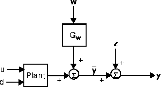
For simplified disturbance modeling:

[Kest,newmod] = smpcest(imod) 
[Kest,newmod] = smpcest(imod,tau,signoise)

Description

In the above block diagram, u is a vector of nu manipulated variables (nu 1), d is a vector of nd measured disturbances (nd 0), w is a vector of unmeasured disturbances, z is measurement noise, y is a vector of outputs, and represents these outputs before the addition of measurement noise. The objective of the state estimator in MPC is to estimate the present and future values of , rejecting as much of the measurement noise as possible. The inputs u and d are assumed perfectly measurable, whereas w and z are unknown and must be inferred from the measurements. Gw is a transfer function matrix representing the effect of each element of w on each output in y.

General Case

imod
Is the model (in mod format) to be used as the basis for the state estimator. It should be the same as that used to calculate the controller gain (see smpccon). It must include a model of the disturbances, i.e., the Gw element in the above diagram. You could, for example, use addumd to combine a plant and disturbance model, yielding a composite model in the proper form.

Q
Is a symmetric, positive semi-definite matrix giving the covariances of the disturbances in w. It must be nw by nw, where nw ( 1) is the number of unmeasured disturbances in imod (i.e., the length of w).

R
Is a symmetric, positive-definite matrix giving the covariances of the measurement noise, z. It must be nym by nym, where nym ( 1) is the number of measured outputs in imod.

The calculated output variable is:

Kest
The estimator gain matrix. It will contain n + ny rows and nym columns, where n is the number of states in imod, and ny is the total number of outputs (measured plus unmeasured).

Simplified disturbance modeling
For the simplified disturbance/noise model we make the following assumptions:

The vectors w, z, y and are all length ny.
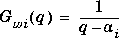
Gw is diagonal. Thus each element of w affects one (and only one) element of y. Diagonal element Gwi has the discrete (sampled-data) form:
where ai = e-T/i, 0 i , and T is the sampling period.

As , Gwi(q) approaches a unity gain, while as , Gwi becomes an integrator.
Element i of w is a stationary white-noise signal with zero mean and standard deviation wi (where wi(k) = wi(k) - wi(k - 1)).
Element i of z is a stationary white-noise signal with zero mean and standard deviation zi.

The input variables are then as follows:

imod
Is the model (in mod format) to be used as the basis for the state estimator. It should be the same as that used to calculate the controller gain (see smpccon).

tau
Is a row vector, length ny, giving the values of i to be used in eq. 1. Each element must satisfy: 0 i . If you use tau=[ ], smpcest uses the default, which is ny zeros.

signoise
Is a row vector, length ny, giving the signal-to-noise ratio for the each disturbance, defined as i = wi =zi. Each element must be nonnegative. If omitted, smpcsim uses an infinite signal-to-noise ratio for each output.

The calculated output variables are:

Kest
The estimator gain matrix.

newmod
The modified version of imod, which must be used in place of imod in any simulation/analysis functions that require Kest (e.g., smpccl, smpcsim, scmpc).

If imod contains n states, and there are n₁ outputs for which i > 0, then newmod will have n + n₁ states. The optimal gain matrix, Kest, will have n + n₁ + ny rows and nym columns. The first n rows will be zero, the next n₁ rows will have the gains for the estimates of the n₁ added states (if any), and the last ny rows will have the gains for estimating the noise-free outputs, .

Examples
Consider the linear system:

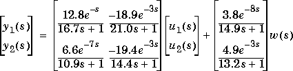
The following statements build two models: pmod, which contains the model of the disturbance, w, and imod, which does not.

g11=poly2tfd(12.8,[16.7 1],0,1);
g21=poly2tfd(6.6,[10.9 1],0,7);
g12=poly2tfd(-18.9,[21.0 1],0,3);
g22=poly2tfd(-19.4,[14.4 1],0,3);
delt=1; ny=2;
imod=tfd2mod(delt,ny,g11,g21,g12,g22);
gw1=poly2tfd(3.8,[14.9 1],0,8);
gw2=poly2tfd(4.9,[13.2 1],0,3);
pmod=addumd(imod,tfd2mod(delt,ny,gw1,gw2));

Calculate the gain for a typical MPC (unconstrained) controller

P=6; M=2; 
ywt=[ ]; uwt=[1 1]; 
Ks=smpccon(imod,ywt,uwt,M,P);

Next design an estimator using the Gw model in pmod. The choices of Q and R are arbitrary. R was made relatively small (since measurement noise will be negligible in the simulations).

Kest1=smpcest(pmod,1,0.001*eye(ny)); 
Ks1=smpccon(pmod,ywt,uwt,M,P);

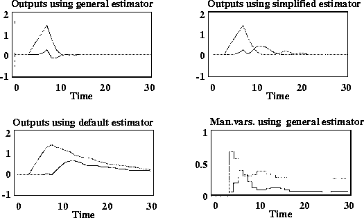
Now design another estimator using a simplified disturbance model in which each output is affected by a disturbance with a first-order time constant of 10 and a signal-to-noise ratio of 3.

tau=[10 10]; signoise=[3 3]; 
[Kest2,newmod]=smpcest(imod,tau,signoise);
Ks2=smpccon(newmod,ywt,uwt,M,P);

Compare the performance of these two estimators to the default (DMC) estimator when there is a unit step in w:

r=[ ]; ulim=[ ]; z=[ ]; d=[ ]; w=[1]; wu=[ ]; tend=30;
[y₁,u1]=smpcsim(pmod,pmod,Ks1,tend,r,ulim,Kest1, z,d,w,wu);
[y₂,u2]=smpcsim(pmod,newmod,Ks2,tend,r,ulim,Kest2, z,d,w,wu);
[y₃,u3]=smpcsim(pmod,imod,Ks,tend,r,ulim,[ ],z,d,w,wu);

The solid lines in the following plots are for y₁ (or u1) and the dashed lines are for y₂ (or u2). Both outputs have setpoints at zero. You can see that the default estimator is much more sluggish than the others in counteracting this type of disturbance. The simplified disturbance design does nearly as well as that using the exact model of the disturbances. The main difference is that it allows more error in y₁ following the disturbance in y₂.

The first 14 states in both imod and pmod are for the response of the outputs to u. Since the unmeasured disturbance has no effect on them, their gains are zero. pmod contains 10 additional disturbance states and there are 2 outputs, so the last 12 rows of Kest1 are nonzero:

Kest1(15:26,:)=
   -0.0556    8.8659
   -0.0594    7.1499
   -0.0635    5.1314
   -0.0679    2.7748
   -0.0725    0.0411
   -0.0781   -0.0182
   -0.0915   -0.0008
   -0.0520    0.0001
    1.2663    0.0000
    0.0281   -0.0000
    0.3137    0.0000
    0.0000    0.9925

and the last 4 rows of Kest2 are nonzero:

Kest2(15:18,:) =
    0.7274         0
         0    0.7274
    0.9261         0
         0    0.9261

Algorithm
In the general case, smpcest uses dlqe2 to calculate the optimal estimator gain, Kest. In the simplified case, it uses an analytical solution of the discrete Riccati equation (which is possible to obtain in this case because the disturbances are independent with low-order dynamics).

The number of rows in Kest is larger than that in newmod because the MPC analysis and simulation functions augment the model states with the outputs (see mpcaugss), and Kest must be set up to account for this.

If all i = 0 and all i = , we get the DMC estimator, which has n rows of zeros followed by an identity matrix of dimension ny. This is the default for all of the MPC analysis and simulation routines that require an estimator gain as input.

Important note:
smpcest decides whether you are using the general case or the simplified approach by checking the number of output arguments you have supplied. If there is only one, it assumes you want the general case. Otherwise, it proceeds as for the simplified case. It checks the dimensions of your input arguments to make sure they are consistent with this decision.

If you get unexpected results or an error message, make sure you have specified the correct number of output arguments.

See Also
scmpc, smpccl, smpccon, smpcsim

smpccon smpcgain, smpcpole