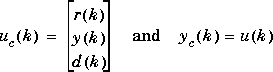
| Model Predictive Control Toolbox | |
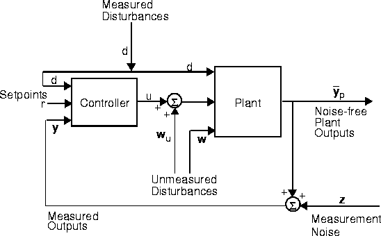
Combines a plant model and a controller model in the MPC mod format, yielding a closed-loop system model in the MPC format. This can be used for stability analysis and linear simulations of closed-loop performance.
Syntax
pmod
Is a model (in the mod format) representing the plant in the above diagram.
imod
Is a model (in the same format) that is to be used to design the MPC controller block shown in the diagram. It may be the same as pmod (in which case there is no model error in the controller design), or it may be different.
Ks
Is a controller gain matrix, which must have been calculated by the function smpccon.
Kest
Is an (optional) estimator gain matrix. If omitted or set to an empty matrix, the default is to use the DMC estimator index DMC estimator. See the documentation for the function smpcest for more details on the design and proper format of Kest.
smpccl
Calculates a model of the closed-loop system, clmod. It is in the mod format and can be used, for example, with analysis functions such as smpcgain and smpcpole, and with simulation routines such as mod2step and dlsimm. smpccl also calculates a model of the controller element, cmod.
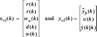
The closed-loop model, clmod, has the following state-space representation:
xcl(k + 1) =  clxcl(k) +
  clucl(k)
ycl(k) = Cclxcl(k) + D clucl(k)
where xcl is a vector of n state variables, ucl is a vector of input variables, ycl is a vector of outputs, and cl, cl, Ccl, and Dcl are matrices of appropriate size. The expert user may want to know the significance of the state variables in xcl. They are (in the following order):
pmod),
imod and the estimator gain, Kest),
 (from the state estimator),
 u signal produced by the standard MPC formulation to yield a u signal that can be used as input to the plant and as a closed-loop output, and
d signal required in the standard MPC formulation. If there are no measured disturbances, these states are omitted.
u signal produced by the standard MPC formulation to yield a u signal that can be used as input to the plant and as a closed-loop output, and
d signal required in the standard MPC formulation. If there are no measured disturbances, these states are omitted.
where  is the estimate of the noise-free plant output at sampling period k based on information available at period k. This estimate is generated by the controller element.
Note that ucl will include d and/or w automatically whenever pmod includes measured disturbances and/or unmeasured disturbances. Thus the length of the ucl vector will depend on the inputs you have defined in pmod and imod. Similarly, ycl depends on the number of outputs and manipulated variables. Let m and p be the lengths of ucl and ycl, respectively. Then
cmod, can be written as:
and the controller states are the same as those of the closed loop system except that the np plant states are not included.
Examples
Consider the linear system:
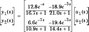
We build this model using the MPC Toolbox functions poly2tfd and tfd2mod.
g11=poly2tfd(12.8,[16.7 1],0,1);
g21=poly2tfd(6.6,[10.9 1],0,7);
g12=poly2tfd(-18.9,[21.0 1],0,3);
g22=poly2tfd(-19.4,[14.4 1],0,3);
delt=3; ny=2;
imod=tfd2mod(delt,ny,g11,g21,g12,g22);
pmod=imod; % No plant/model mismatch
M < P: We specify the defaults for the other tuning parameters, uwt and ywt, then calculate the controller gain:
P=6; % Prediction horizon. M=2; % Number of moves (input horizon).ywt=[ ]; % Output weights (default - unity on % all outputs).uwt=[ ]; % Man. Var weights (default - zero on % all man. vars).Ks=smpccon(imod,ywt,uwt,M,P);
You can also use the closed-loop model to calculate and plot the step response with respect to all the inputs. The appropriate commands are:
Since the closed-loop system has m = 6 inputs and p = 6 outputs, only one of the plots is reproduced here. It shows the response of the first 4 closed-loop outputs to a step in the first closed-loop input, which is the setpoint for y1: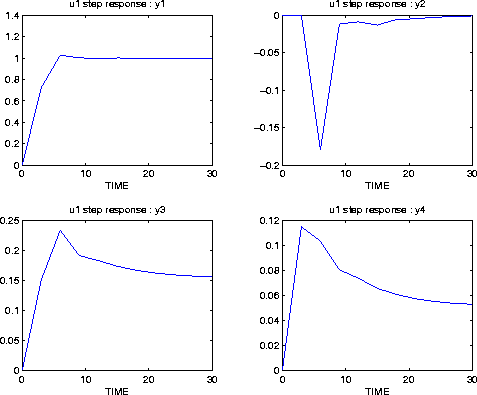
Closed-loop outputs y1 and y2 are the true plant outputs (noise-free). Output y1 goes to the new setpoint quickly with a small overshoot. This causes a small, short-term disturbance in y2. The plots for y3 and y4 show the required variation in the manipulated variables.
The following commands show how you could use dlsimm to calculate the response of the closed-loop system to a step in the setpoint for y1, with added random measurement noise.
r=[ones(11,1) zeros(11,1)];
z=0.1*rand(11,2);
wu=zeros(11,2);
d=[ ];
w=[ ];
ucl=[r z wu d w];
[phicl,gamcl,ccl,dcl]=mod2ss(clmods);
ycl=dlsimm(phicl,gamcl,ccl,dcl,ucl);
y=ycl(:,1:2); u=ycl(:,3:4); ym=ycl(:,5:6);
Restrictions
imod and pmod must have been created using the same sampling period, and an equal number of outputs, measured disturbances, and manipulated variables.
imod and pmod must be strictly proper, i.e., the D matrices in their state-space descriptions must be zero. Exception: the last nw columns of the D matrices may be nonzero, i.e., the unmeasured disturbance may have an immediate effect on the outputs.
See Also
mod2step, scmpc, smpccon, smpcest, smpcgain, smpcpole, smpcsim
| sermod | smpccon | |