Model Predictive Control Toolbox

Simulates closed-loop systems with hard bounds on manipulated variables and/or outputs using models in the MPC mod format. Solves the MPC optimization problem by quadratic programming.

Syntax

• yp = scmpc(pmod,imod,ywt,uwt,M,P,tend,r) 
  [yp,u,ym] = scmpc(pmod,imod,ywt,uwt,M,P,tend, ... 
     r,ulim,ylim,Kest,z,d,w,wu) 
  

Description

scmpc simulates the performance of the type of system shown in the above diagram when there are bounds on the manipulated variables and/or outputs.

The required input variables are as follows:

pmod
Is a model in the MPC mod format that is to represent the plant.

imod
Is a model in the MPC mod format that is to be used for state estimation in the controller. In general, it can be different from pmod if you want to simulate the effect of plant/controller model mismatch.

ywt
Is a matrix of weights that will be applied to the setpoint tracking errors (optional). If ywt=[ ], the default is equal (unity) weighting of all outputs over the entire prediction horizon. If ywt[ ], it must have ny columns, where ny is the number of outputs. All weights must be 0.

You may vary the weights at each step in the prediction horizon by including up to P rows in ywt. Then the first row of ny values applies to the tracking errors in the first step in the prediction horizon, the next row applies to the next step, etc. See smpccon for details on the form of the optimization objective function.

If you supply only nrow rows, where 1 nrow < P, scmpc will use the last row to fill in any remaining steps. Thus if you wish the weighting to be the same for all P steps, you need only specify a single row.

uwt
Is as for ywt, except that uwt applies to the changes in the manipulated variables. If you use uwt=[ ], the default is zero weighting. If uwt[ ], it must have nu columns, where nu is the number of manipulated variables.

M
There are two ways to specify this variable:

If it is a scalar, scmpc interprets it as the input horizon (number of moves) as in DMC.

If it is a row vector containing nb elements, each element of the vector indicates the number of steps over which u = 0 during the optimization and scmpc interprets it as a set of nb blocking factors. There may be 1 nb P blocking factors, and their sum must be P.

If you set M=[ ], the default is M=P, which is equivalent to M=ones(1,P).

P
The number of sampling periods in the prediction horizon.

tend
Is the desired duration of the simulation (in time units).

r
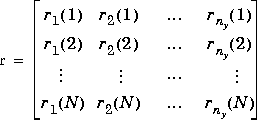
Is a setpoint matrix consisting of N rows and ny columns, where ny is the number of output variables, y:

where ri(k) is the setpoint for output j at time t = kT, and T is the sampling period (as specified by the minfo vector in the mod format of pmod and imod). If tend > NT, the setpoints vary for the first N periods in the simulation, as specified by r, and are then held constant at the values given in the last row of r for the remainder of the simulation.

In many simulations one wants the setpoints to be constant for the entire time, in which case r need only contain a single row of ny values.

If you set r=[ ], the default is a row of ny zeros.

The following input variables are optional. In general, setting one of them equal to an empty matrix causes scmpc to use the default value, which is given in the description.

ulim

Is a matrix giving the limits on the manipulated variables. Its format is as follows:

Note that it contains three matrices of N rows. In this case, the limits on N are 1 N nb, where nb is the number of times the manipulated variables are to change over the input horizon. If you supply fewer than nb rows, the last row is repeated automatically.

    The first matrix specifies the lower bounds on the nu manipulated variables. For example, umin,j(2) is the lower bound for manipulated variable j for the second move of the manipulated variables (where the first move is at the start of the prediction horizon). If umin,j(k) = -inf, manipulated variable j will have no lower bound for that move.

    The second matrix gives the upper bounds on the manipulated variables. If umax,j(k) = inf, manipulated variable j will have no upper bound for that move.

    The lower and upper bounds may be either positive or negative (or zero) as long as umin,j(k) umax,j(k).

    The third matrix gives the limits on the rate of change of the manipulated variables. In other words, cmpc will force|uj(k) - uj(k - 1)| umax,j(k). The limits on the rate of change must be nonnegative and finite. If you want it to be unbounded, set the bound to a large number (but not too large -- a value of 10⁶ should work well in most cases).

    The default is umin = -inf, umax = inf and umax = 10⁶

ylim
Same format as for ulim, but for the lower and upper bounds of the outputs. The first row applies to the first point in the prediction horizon. The default is ymin = -inf, and ymax = inf.

Kest
Is the estimator gain matrix. The default is the DMC estimator. See smpcest for more details.

z
Is measurement noise that will be added to the outputs (see above diagram). The format is the same as for r. The default is a row of ny zeros.

d
Is a matrix of measured disturbances (see above diagram). The format is the same as for r, except that the number of columns is nd rather than ny. The default is a row of nd zeros.s

w
Is a matrix of unmeasured disturbances (see above diagram). The format is the same as for r, except that the number of columns is nw rather than ny.The default is a row of nw zeros.

wu
Is a matrix of unmeasured disturbances that are added to the manipulated variables (see above diagram). The format is the same as for r, except that the number of columns is nu rather than ny. The default is a row of nu zeros.

Notes

• You may use a different number of rows in the matrices r, z, d, w and wu, should that be appropriate for your simulation.
• The ulim constraints used here are fundamentally different from the usat constraints used in the smpcsim function. The ulim constraints are defined relative to the beginning of the prediction horizon, which moves as the simulation progresses. Thus at each sampling period, k, the ulim constraints apply to a block of calculated moves that begin at sampling period k and extend for the duration of the input horizon. The usat constraints, on the other hand, are relative to the fixed point t = 0, the start of the simulation.

yp
Is a matrix containing M rows and ny columns, where M = max(fix(tend/T) + 1, 2). The first row will contain the initial condition, and row k - 1 will give the values of the noise-free plant outputs, (see above diagram), at time t = kT.

u
Is a matrix containing the same number of rows as yp and nu columns. The time corresponding to each row is the same as for yp. The elements in each row are the values of the manipulated variables, u (see above diagram).

Note
The u values are those coming from the controller before the addition of the unmeasured disturbance, wu.

ym
Is a matrix of the same structure as yp, containing the values of the predicted output from the state estimator in the controller. These will, in general, differ from those in yp if imodpmod and/or there are unmeasured disturbances. The prediction includes the effect of the most recent measurement, i.e., it is .

For unconstrained problems, scmpc and smpcsim should give the same results. The latter will be faster because it uses an analytical solution of the QP problem, whereas scmpc solves it by iteration.

Examples
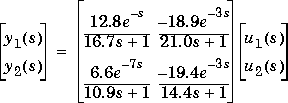
Consider the linear system:

The following statements build the model and set up the controller in the same way as in the smpcsim example.

• g11=poly2tfd(12.8,[16.7 1],0,1);
  g21=poly2tfd(6.6,[10.9 1],0,7);
  g12=poly2tfd(-18.9,[21.0 1],0,3);
  g22=poly2tfd(-19.4,[14.4 1],0,3);
  delt=3; ny=2; 
  imod=tfd2mod(delt,ny,g11,g21,g12,g22); 
  pmod=imod; P=6; M=2; ywt=[ ]; uwt=[1 1]; 
  tend=30; r=[0 1];
  

• ulim=[-inf -0.15 inf inf 0.1 100]; 
  ylim=[ ]; 
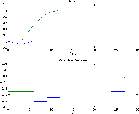
  [y,u]=scmpc(pmod,imod,ywt,uwt,M,P,tend,r,ulim,ylim); 
  plotall(y,u,delt), pause
  

We next apply a lower bound of zero to both outputs:

• ulim=[-inf -0.15 inf inf 0.1 100]; 
  ylim=[0 0 inf inf]; 
  [y,u]=scmpc(pmod,imod,ywt,uwt,M,P,tend,r,ulim,ylim);
  plotall(y,u,delt),
  pause
  

Restrictions

• Initial conditions of zero are used for all states in imod and pmod. This simulates the condition where all variables represent a deviation from a steady-state initial condition.
• The first nu + nd columns of the D matrices in imod and pmod must be zero. In other words, neither u nor d may have an immediate effect on the outputs.

Suggestions
Problems with many inequality constraints can be very time consuming. You can minimize the number of constraints by:

• Using small values for P and/or M.
• Leaving variables unconstrained (limits at ±inf) intermittently unless you think the constraint is important.

See Also
plotall, ploteach, smpccl, smpccon, smpcest, smpcsim

poly2tfd, poly format

sermod