GARCH Toolbox

crosscorr

Plot or return computed sample cross-correlation function

Syntax

• crosscorr(Series1, Series2, nLags, nSTDs)
  [XCF, Lags, Bounds] = crosscorr(Series1, Series2, nLags, nSTDs)
  

Arguments

Series1	Vector of observations of the first univariate time series for which crosscorr computes or plots the sample cross-correlation function (XCF). The last element of Series1 contains the most recent observation.
Series2	Vector of observations of the second univariate time series for which crosscorr computes or plots the sample XCF. The last element of Series2 contains the most recent observation.
nLags	(optional) Positive, scalar integer indicating the number of lags of the XCF to compute. If nLags = [] or is not specified, crosscorr computes the XCF at lags 0, ±1, ±2, ..., ±T, where T = min([20, min([length(Series1), length(Series2)])-1]).
nSTDs	(optional) Positive scalar indicating the number of standard deviations of the sample XCF estimation error to compute, if Series1 and Series2 are uncorrelated. If nSTDs = [] or is not specified, the default is 2 (i.e., approximate 95 percent confidence interval).

Description

crosscorr(Series1, Series2, nLags, nSTDs) computes and plots the sample cross-correlation function (XCF) between two univariate, stochastic time series. To plot the XCF sequence without the confidence bounds, set nSTDs = 0.

[XCF, Lags, Bounds] = crosscorr(Series1, Series2, nLags, nSTDs) computes and returns the XCF sequence.

XCF	Sample cross-correlation function between Series1 and Series2. XCF is a vector of length 2(nLags)+1 corresponding to lags 0, ±1, ±2, ..., ±nLags. The center element of XCF contains the 0th lag cross correlation. XCF is a row (column) vector if Series1 is a row (column) vector.
Lags	Vector of lags corresponding to XCF(-nLags, ..., +nLags).
Bounds	Two-element vector indicating the approximate upper and lower confidence bounds assuming Series1 and Series2 are completely uncorrelated.

Example

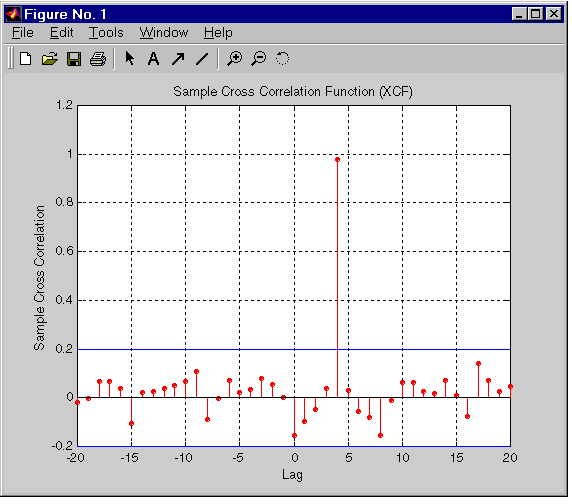
Create a random sequence of 100 Gaussian deviates, and a delayed version lagged by four samples. Compute the XCF, and then plot it to see the XCF peak at the fourth lag.

• randn('state',100)              % Start from a known state.
  x           = randn(100,1);     % 100 Gaussian deviates, N(0,1).
  y           = lagmatrix(x, 4);  % Delay it by 4 samples.
  y(isnan(y)) = 0;                % Replace NaNs with zeros.
  [XCF, Lags, Bounds] = crosscorr(x,y);  % Compute the XCF with
                                         % 95 percent confidence.
  [Lags, XCF]
  
  ans =
  
    -20.0000   -0.0210
    -19.0000   -0.0041
    -18.0000    0.0661
    -17.0000    0.0668
    -16.0000    0.0380
    -15.0000   -0.1060
    -14.0000    0.0235
    -13.0000    0.0240
    -12.0000    0.0366
    -11.0000    0.0505
    -10.0000    0.0661
     -9.0000    0.1072
     -8.0000   -0.0893
     -7.0000   -0.0018
     -6.0000    0.0730
     -5.0000    0.0204
     -4.0000    0.0352
     -3.0000    0.0792
     -2.0000    0.0550
     -1.0000    0.0004
           0   -0.1556
      1.0000   -0.0959
      2.0000   -0.0479
      3.0000    0.0361
      4.0000    0.9802
      5.0000    0.0304
      6.0000   -0.0566
      7.0000   -0.0793
      8.0000   -0.1557
      9.0000   -0.0128
     10.0000    0.0623
     11.0000    0.0625
     12.0000    0.0268
     13.0000    0.0158
     14.0000    0.0709
     15.0000    0.0102
     16.0000   -0.0769
     17.0000    0.1410
     18.0000    0.0714
     19.0000    0.0272
     20.0000    0.0473
  
  Bounds =
  
      0.2000
     -0.2000
  
  crosscorr(x,y)         % Use the same example, but plot the XCF 
                         % sequence. Note the peak at the 4th lag.
  
  
  

See Also
autocorr, parcorr

filter (in the online MATLAB Function Reference)

autocorr

garchar