Filter Design Issues (Using the Communications Blockset)

Communications Blockset

Filter Design Issues

After demodulating, you might want to filter out the carrier signal, especially if you are using passband simulation. The Signal Processing Toolbox provides functions that can help you design your filter, such as butter, cheby1, cheby2, and ellip. Different demodulation methods have different properties, and you might need to test your application with several filters before deciding which is most suitable. This section mentions two issues that relate to the use of filters: cutoff frequency and time lag.

Example: Varying the Filter's Cutoff Frequency

In many situations, a suitable cutoff frequency is half the carrier frequency. Since the carrier frequency must be higher than the bandwidth of the message signal, a cutoff frequency chosen in this way limits the bandwidth of the message signal. If the cutoff frequency is too high, the carrier frequency may not be filtered out. If the cutoff frequency is too low, it might narrow the bandwidth of the message signal.

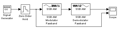
The following example modulates a sawtooth message signal, demodulates the resulting signal using a Butterworth filter, and plots the original and recovered signals. The Butterworth filter is implemented within the SSB AM Demodulator Passband block.

Before building the model, first execute this command at the MATLAB prompt:

```
[num,den] = butter(2,25*.01);
```

Here, 2 is the order of the Butterworth filter, 25 is the carrier signal frequency, and .01 is the sample time of the signal in Simulink. The variables num and den represent the numerator and denominator, respectively, of the filter's transfer function. These variables reside in the MATLAB workspace, where Simulink can access them during the simulation. The butter function is in the Signal Processing Toolbox.

Now to open the completed model, click here in the MATLAB Help browser. To build the model, gather and configure these blocks:

Signal Generator, in the Simulink Sources library

Set Wave form to Sawtooth.

Set Amplitude to 4.

Set Frequency to .3.

Zero-Order Hold, in the Simulink Discrete library

Set Sample time to .01.

SSB AM Modulator Passband, in the Analog Passband sublibrary of the Modulation library

Set Carrier frequency to 25.

Set Time delay for Hilbert transform filter to .1.

Set Sample time to .01.

SSB AM Demodulator Passband, in the Analog Passband sublibrary of the Modulation library

Set Carrier frequency to 25.

Set Lowpass filter numerator to num.

Set Lowpass filter denominator to den.

Set Sample time to .01.

Scope, in the Simulink Sinks library

After double-clicking on the block to open it, click the Parameters icon and set Number of axes to 2.

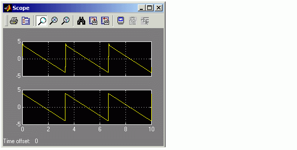
Connect the blocks as in the figure. Also, from the model window's Simulation menu, choose Simulation parameters; then in the Simulation Parameters dialog box, set Stop time to 10. Running the model produces the following scope image. The image reflects the original and recovered signals, with a moderate filter cutoff.

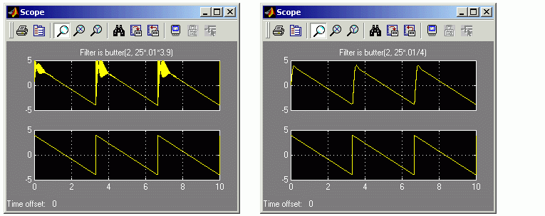
Other Filter Cutoffs. To see the effect of a lowpass filter with a higher cutoff frequency, type

```
[num,den] = butter(2,25*.01*3.9);
```

at the MATLAB prompt and then run the simulation again. The new result is the left image in the following figure. The higher cutoff frequency allows the carrier signal to interfere with the demodulated signal.

To see the effect of a lowpass filter with a lower cutoff frequency, type

```
[num,den] = butter(2,25*.01/4);
```

at the MATLAB prompt and then run the simulation again. The new result is the right image in the figure below. The lower cutoff frequency narrows the bandwidth of the demodulated signal.

Example: Time Lag from Filtering

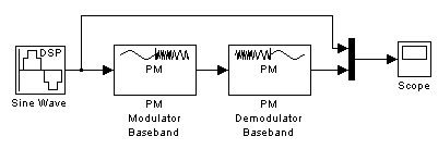
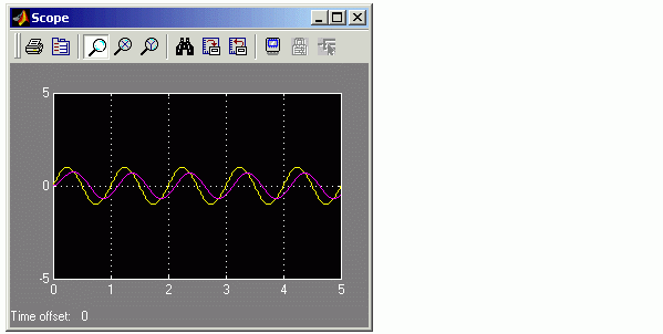
There is invariably a delay between a demodulated signal and the original received signal. Both the filter order and the filter parameters directly affect the length of this delay. The following example illustrates the delay by plotting a signal before modulation and after demodulation. The curve with amplitude 1 is the original sine wave and the other curve is the recovered signal.

To open the completed model, click here in the MATLAB Help browser. To build the model, gather and configure these blocks:

Sine Wave, in the DSP Blockset DSP Sources library (not the Sine Wave block in the Simulink Sources library)

Set Frequency to 1

PM Modulator Baseband, in the Analog Baseband sublibrary of the Modulation library. Use default parameters.

PM Demodulator Baseband, in the Analog Baseband sublibrary of the Modulation library. Use default parameters.

Mux, in the Simulink Signals & Systems library

Scope, in the Simulink Sinks library

Connect the blocks as in the figure. Also, from the model window's Simulation menu, choose Simulation parameters; then in the Simulation Parameters dialog box, set Stop time to 5. Running the model produces the following scope image.

Timing Issues in Analog Modulation Digital Modulation