| Robust Control Toolbox | |
System realization via Hankel singular value decomposition.
Syntax
[a,b,c,d,totbnd,svh] = imp2ss(y)
[a,b,c,d,totbnd,svh] = imp2ss(y,ts,nu,ny,tol)
[ss,totbnd,svh] = imp2ss(imp)
[ss,totbnd,svh] = imp2ss(imp,tol)
Description
The function imp2ss produces an approximate state-space realization of a given impulse response
bilin) if t is positive; otherwise a discrete-time realization is returned. In the SISO case the variable y is the impulse response vector; in the MIMO case y is a N+1-column matrix containing N + 1 time samples of the matrix-valued impulse response H0, ..., HN of an nu-input, ny-output system stored row wise:
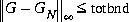
The variable tol bounds the H norm of the error between the approximate realization (a, b, c, d) and an exact realization of y; the order, say n, of the realization (a, b, c, d) is determined by the infinity norm error bound specified by the input variable tol. The inputs
 ts, nu, ny, tol are optional; if not present they default to the values ts = 0, nu = 1, ny = (no. of rows of y)/nu,  . The output
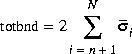
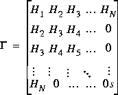
 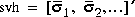 returns the singular values (arranged in descending order of magnitude) of the Hankel matrix:
Denoting by GN a high-order exact realization of y, the low-order approximate model G enjoys the H norm bound
Algorithm
The realization (a, b, c, d) is computed using the Hankel SVD procedure proposed by Kung [2] as a method for approximately implementing the classical Hankel factorization realization algorithm. Kung's SVD realization procedure was subsequently shown to be equivalent to doing balanced truncation (balmr) on an exact state space realization of the finite impulse response {y(1),....y(N)} [3]. The infinity norm error bound for discrete balanced truncation was later derived by Al-Saggaf and Franklin [1]. The algorithm is as follows:
 from the data y.
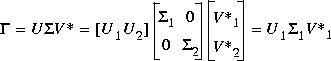
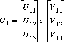
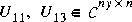
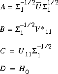
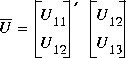
 1 has dimension n x n and the entries of 2 are nearly zero. U1 and V1 have ny and nu columns, respectively.
 and
and 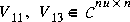 .
.

See Also
ohklmr, schmr, balmr, bstschmr
References
[1] U. M. Al-Saggaf and G. F. Franklin, "An Error Bound for a Discrete Reduced Order Model of a Linear Multivariable System," IEEE Trans. on Autom. Contr., AC-32, pp. 815-819, 1987.
[2] S. Y. Kung, "A New Identification and Model Reduction Algorithm via Singular Value Decompositions," Proc.Twelth Asilomar Conf. on Circuits, Systems and Computers., pp. 705-714, November 6-8, 1978.
[3] L. M. Silverman and M. Bettayeb, "Optimal Approximation of Linear Systems," Proc. American Control Conf., San Francisco, CA, 1980.
| hinfopt | interc | |