SimPowerSystems

Frequency Analysis

The Measurements library of powerlib contains an Impedance Measurement block that measures the impedance between any two nodes of a circuit. In the following two sections you measure the impedance of your circuit between bus B2 and ground by using two methods:

• Calculation from the state space model
• Automatic measurement using the Impedance Measurement block and the Powergui block

Obtaining the Impedance vs. Frequency from the State-Space Model

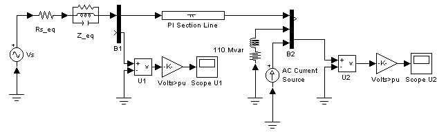
To measure the impedance versus frequency at bus bar B2, you will need a current source at bus bar B2 providing a second input to the state-space model. Open the Electrical Sources library and copy the AC Current Source block into your model. Connect this source at bus bar B2, as shown below. Set the current source magnitude to 0 and keep its frequency at 60 Hz. Rearrange the blocks as follows:

Figure 1-2: AC Current Source at the B2 Bus Bar

Now compute the state-space representation of the model circuitl with the power2sys function. Enter the following command at the MATLAB prompt.

• [A,B,C,D,x0,states,inputs,outputs]=power2sys('circuitl');
  

The power2sys function returns the state-space model of your circuit in the four matrices A, B, C, and D. x0 is the vector of initial conditions that you have just displayed with the Powergui block. The names of the state variables, inputs, and outputs are returned in three string matrices.

• states =
  
  Il_110 Mvars
  Uc_input PI Section Line
  Il_ sect1 PI Section Line
  Uc_output PI Section Line
  Il_Z_eq
  Uc_Z_eq
  
  inputs =
  
  U_Vs
  I_AC Current Source
  
  outputs =
  
  U_U1
  U_U2
  

Note that you could have obtained the names and ordering of the states, inputs and outputs directly from the Powergui block.

Once the state-space model of the system is known, it can be analyzed in the frequency domain. For example, the modes of this circuit can be found from the eigenvalues of matrix A (use the MATLAB eig command).

• eig(A)
  ans =
  1.0e+05 *
  -2.4972          
  -0.0001 + 0.0144i <---229 Hz
  -0.0001 - 0.0144i
  -0.0002 + 0.0056i <---89 Hz
  -0.0002 - 0.0056i
  -0.0000
  

This system has two oscillatory modes at 89 Hz and 229 Hz. The 89 Hz mode is due to the equivalent source, which is modeled by a single pole equivalent. The 229 Hz mode is the first mode of the line modeled by a single PI section.

If you own the Control System Toolbox, you can compute the impedance of the network as a function of frequency by using the bode function.

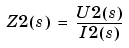
In the Laplace domain, the impedance Z2 at bus B2 is defined as the transfer function between the current injected at bus B2 (input 2 of the system) and the voltage measured at bus B2 (output 2 of the system):

The impedance at bus B2 for the 0-1500Hz range can be calculated and visualized as follows:

• freq=0:1500;
  w=2*freq;
  [mag1,phase1]=bode(A,B,C,D,2,w);
  semilogy(freq,mag1(:,2));
  

Repeat the same process to get the frequency response with a 10 section line model. Open the PI Section Line dialog box and change the number of sections from 1 to 10. To calculate the new frequency response and superimpose it upon the one obtained with a single line section, enter the following commands:

• [A,B,C,D]=power2sys('circuit1');
  [mag10,phase10]=bode(A,B,C,D,2,w);
  semilogy(freq,mag1(:,2),freq,mag10(:,2));
  

This is the resulting plot.

Figure 1-3: Impedance at Bus B2 as Function of Frequency

This graph indicates that the frequency range represented by the single line section model is limited to approximately 150 Hz. For higher frequencies, the 10 line section model is a better approximation.

For a distributed parameter line model the propagation speed is

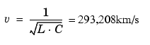
The propagation time for 300 km is therefore T=300/293,208=1.023 ms and the frequency of the first line mode is f1=1/4T=244 Hz. A distributed parameter line would have an infinite number of modes every 244 + n * 488 Hz (n = 1, 2, 3...). The 10 section line model simulates the first 10 modes. The first three line modes can be seen in Figure 1-3. (244Hz, 732Hz, and 1220 Hz).

Obtaining the Impedance vs Frequency from the Impedance Measurement Block and the Powergui Block

The process described above to measure a circuit impedance has been automated in the Power System Blockset. Open the Measurements library of powerlib, copy the Impedance Measurement block into your model, and rename it ZB2. The block uses a current source and a voltage measurement to perform the impedance measurement. Connect the two inputs of this block between bus bar B2 and ground as shown.

Figure 1-4: Measuring Impedance vs Frequency with the Impedance Measurement Block

Now open the powergui. In the Tools menu, select Impedance vs Frequency Measurement. A new window opens, showing the list of Impedance Measurement blocks available in your circuit.

In your case, only one impedance is measured, and it is identified by ZB2 (the name of the ZB2 block) in the window. Fill in the frequency range by entering 0:2:1500 (zero to 1500 Hz by steps of 2 Hz). Select the logarithmic scale to display Z magnitude. Check the Save data to workspace button and enter ZB2 as the variable name that will contain the impedance vs frequency. Click the Display button.

When the calculation is finished, a graphic window appears with the magnitude and phase as functions of frequency. The magnitude should be identical to the plot (for one line section) shown in Figure 1-3. If you look in your workspace, you should have a variable named ZB2. It is a two-column matrix containing frequency in column 1 and complex impedance in column 2.

Now open the Simulation --> Simulation parameters dialog of your circuit1 model. On the Solver pane, select the ode23tb integration algorithm. Set the relative tolerance to 1e-4 and keep auto for the other parameters. Set the stop time to 0.05. Open the scopes and start the simulation.

Look at the waveforms of the sending and receiving end voltages on ScopeU1 and ScopeU2. As the state variables have been automatically initialized, the system starts in steady state and sinusoidal waveforms are observed.

Finally open the powergui. In the Tools menu select Initial Values of State Variables --> Display or Modify Initial State Value and reset all the states to 0 by selecting the Reset to zero button and then the Apply button. Restart the simulation and observe the transient when the line is energized from 0.

Figure 1-5: Receiving End Voltage U2 with 10 PI Section Line

Steady-State Analysis

Session 3: Simulating Transients