| Partial Differential Equation Toolbox | |
The Elliptic Equation
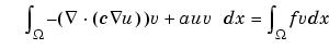
The basic elliptic equation handled by the toolbox is
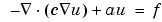 in
in 
where is a bounded domain in the plane. c, a, f, and the unknown solution u are complex functions defined on . c can also be a 2-by-2 matrix function on . The boundary conditions specify a combination of u and its normal derivative on the boundary:
 .
.
 · (c
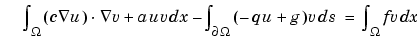
· (c u) + qu = g on
  .
.
 is the outward unit normal. g, q, h, and r are functions defined on
  .
.
Our nomenclature deviates slightly from the tradition for potential theory, where a Neumann condition usually refers to the case q = 0 and our Neumann would be called a mixed condition. In some contexts, the generalized Neumann boundary conditions is also referred to as the Robin boundary conditions. In variational calculus, Dirichlet conditions are also called essential boundary conditions and restrict the trial space. Neumann conditions are also called natural conditions and arise as necessary conditions for a solution. The variational form of the PDE Toolbox equation with Neumann conditions is given below.
The approximate solution to the elliptic PDE is found in three steps:
and the boundary conditions. This can be done either interactively using pdetool (see The Graphical User Interface) or through M-files (see pdegeom and pdebound.)
. The toolbox has mesh generating and mesh refining facilities. A mesh is described by three matrices of fixed format that contain information about the mesh points, the boundary segments, and the triangles.
More elaborate applications make use of the Finite Element Method (FEM) specific information returned by the different functions of the toolbox. Therefore we quickly summarize the theory and technique of FEM solvers to enable advanced applications to make full use of the computed quantities.
FEM can be summarized in the following sentence: Project the weak form of the differential equation onto a finite-dimensional function space. The rest of this section deals with explaining the above statement.
We start with the weak form of the differential equation. Without restricting the generality, we assume generalized Neumann conditions on the whole boundary, since Dirichlet conditions can be approximated by generalized Neumann conditions. In the simple case of a unit matrix h, setting g = qr and then letting  yields the Dirichlet condition because division with a very large q cancels the normal derivative terms. The actual implementation is different, since the above procedure may create conditioning problems. The mixed boundary condition of the system case requires a more complicated treatment, described in the section The Elliptic System
Assume that u is a solution of the differential equation. Multiply the equation with an arbitrary test function v and integrate on :
Integrate by parts (i.e., use Green's formula) to obtain
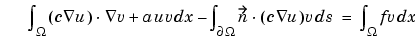
The boundary integral can be replaced by the boundary condition:
Replace the original problem with Find u such that

This equation is called the variational, or weak, form of the differential equation. Obviously, any solution of the differential equation is also a solution of the variational problem. The reverse is true under some restrictions on the domain and on the coefficient functions. The solution of the variational problem is also called the weak solution of the differential equation.
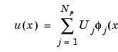
The solution u and the test functions v belong to some function space V. The next step is to choose an Np-dimensional subspace  . Project the weak form of the differential equation onto a finite-dimensional function space simply means requesting u and v to lie in
 rather than V. The solution of the finite dimensional problem turns out to be the element of
  that lies closest to the weak solution when measured in the energy norm (see below). Convergence is guaranteed if the space
  tends to V as
  . Since the differential operator is linear, we demand that the variational equation is satisfied for Np test-functions
  i
i 
 that form a basis, i.e.,

and obtain the system of equations
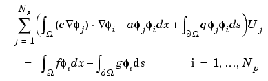
and rewrite the system in the form (K + M + Q)U = F + G.
K, M, and Q are Np-by-Np matrices, and F and G are Np-vectors. K, M, and F are produced by assema, while Q, G are produced by assemb. When it is not necessary to distinguish K, M, and Q or F and G, we collapse the notations to
KU = F, which form the output of assempde.
When the problem is self-adjoint and elliptic in the usual mathematical sense, the matrix K + M + Q becomes symmetric and positive definite. Many common problems have these characteristics, most notably those that can also be formulated as minimization problems. For the case of a scalar equation, K, M, and Q are obviously symmetric. If c(x) 
 > 0, a(x) 0 and q(x) 0 with q(x) > 0 on some part of
  , then, if U
  0.
0.

UT(K + M + Q)U is the energy norm. There are many choices of the test-function spaces. The toolbox uses continuous functions that are linear on each triangle of the mesh. Piecewise linearity guarantees that the integrals defining the stiffness matrix K exist. Projection onto  is nothing more than linear interpolation, and the evaluation of the solution inside a triangle is done just in terms of the nodal values. If the mesh is uniformly refined,
  approximates the set of smooth functions on .
A suitable basis for  is the set of "tent" or "hat" functions i. These are linear on each triangle and take the value 0 at all nodes xj except for xi. Requesting i(xi) = 1 yields the very pleasant property
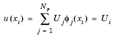
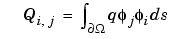
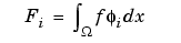
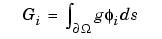
I.e., by solving the FEM system we obtain the nodal values of the approximate solution. Finally note that the basis function i vanishes on all the triangles that do not contain the node xi. The immediate consequence is that the integrals appearing in Ki,j, Mi,j, Qi,j, Fi and Gi only need to be computed on the triangles that contain the node xi. Secondly, it means that Ki,j and Mi,j are zero unless xi and xj are vertices of the same triangle and thus K and M are very sparse matrices. Their sparse structure depends on the ordering of the indices of the mesh points.
The integrals in the FEM matrices are computed by adding the contributions from each triangle to the corresponding entries (i.e., only if the corresponding mesh point is a vertex of the triangle). This process is commonly called assembling, hence the name of the function assempde.
The assembling routines scan the triangles of the mesh. For each triangle they compute the so-called local matrices and add their components to the correct positions in the sparse matrices or vectors. (The local 3-by-3 matrices contain the integrals evaluated only on the current triangle. The coefficients are assumed constant on the triangle and they are evaluated only in the triangle barycenter.) The integrals are computed using the mid-point rule. This approximation is optimal since it has the same order of accuracy as the piecewise linear interpolation.
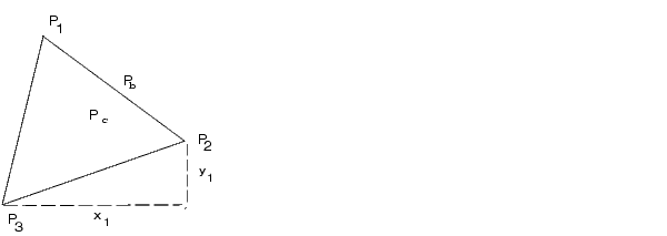
Consider a triangle given by the nodes P1, P2, and P3 as in the following figure.
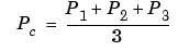
The simplest computations are for the local mass matrix m:

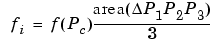
where Pc is the center of mass of  P1P2P3, i.e.,
The contribution to the right side F is just
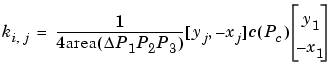
For the local stiffness matrix we have to evaluate the gradients of the basis functions that do not vanish on P1P2P3. Since the basis functions are linear on the triangle P1P2P3, the gradients are constants. Denote the basis functions 1, 2, and 3 such that i(Pi) = 1. If P2 - P3 = [x1,y1]T then we have that
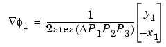
and after integration (taking c as a constant matrix on the triangle)
If two vertices of the triangle lie on the boundary  , they contribute to the line integrals associated to the boundary conditions. If the two boundary points are P1 and P2, then we have
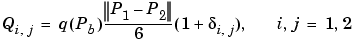
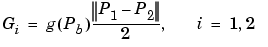
where Pb is the midpoint of P1P2.
For each triangle the vertices Pm of the local triangle correspond to the indices im of the mesh points. The contributions of the individual triangle are added to the matrices such that, e.g.,

This is done by the function assempde. The gradients and the areas of the triangles are computed by the function pdetrg.
The Dirichlet boundary conditions are treated in a slightly different manner. They are eliminated from the linear system by a procedure that yields a symmetric, reduced system. The function assempde can return matrices K, F, B, and ud such that the solution is u = Bv + ud where Kv = F. u is an Np-vector, and if the rank of the Dirichlet conditions is rD, then v has Np - rD components.
| | The Finite Element Method | The Elliptic System | |

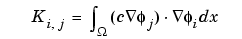 (Stiffness matrix)
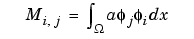 (Mass matrix)