Partial Differential Equation Toolbox

Boundary Menu

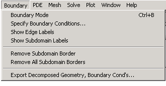
Boundary Mode	Enter the boundary mode.
Specify Boundary Conditions . . .	Specify boundary conditions for the selected boundaries. If no boundaries are selected, the entered boundary condition applies to all boundaries.
Show Edge Labels	Toggle the labeling of the edges (outer boundaries and subdomain borders) on/off. The edges are labeled using the column number in the Decomposed Geometry matrix.
Show Subdomains Labels	Toggle the labeling of the subdomains on/off. The subdomains are labeled using the subdomain numbering in the Decomposed Geometry matrix.
Remove Subdomain Border	Remove selected subdomain borders.
Remove All Subdomain Borders	Remove all subdomain borders.
Export Decomposed Geometry, Boundary Cond's . . .	Export the Decomposed Geometry matrix g and the Boundary Condition matrix b to the main workspace.

Specify Boundary Conditions . . .

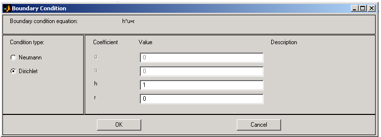
Specify boundary conditions . . . displays a dialog box in which you can specify the boundary condition for the selected boundary segments. There are three different condition types:

• Generalized Neumann conditions, where the boundary condition is determined by the coefficients q and g according to the following equation:

• In the system cases, q is a 2-by-2 matrix and g is a 2-by-1 vector.

• Dirichlet conditions: u is specified on the boundary. The boundary condition equation is hu = r, where h is a weight factor that can be applied (normally 1).

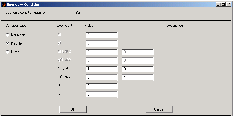
• In the system cases, h is a 2-by-2 matrix and r is a 2-by-1 vector.

• Mixed boundary conditions (system cases only), which is a mix of Dirichlet and Neumann conditions. q is a 2-by-2 matrix, g is a 2-by-1 vector, h is a 1-by-2 vector, and r is a scalar.

The following figure shows the boundary condition dialog box for the generic system PDE.

For boundary condition entries you can use the following variables in a valid MATLAB expression:

• The 2-D coordinates x and y.
• A boundary segment parameter s, proportional to arc length. s is 0 at the start of the boundary segment and increases to 1 along the boundary segment in the direction indicated by the arrow.
• The outward normal vector components nx and ny. If you need the tangential vector, it can be expressed using nx and ny since tx = -ny and ty = nx.
• The solution u.
• The time t.

Note    If the boundary condition is a function of the solution u, you must use the nonlinear solver. If the boundary condition is a function of the time t, you must choose a parabolic or hyperbolic PDE.

Examples: (100-80*s).*nx, and cos(x.^2)

In the nongeneric application modes, the Description column contains descriptions of the physical interpretation of the boundary condition parameters.

Draw Menu

PDE Menu