Partial Differential Equation Toolbox

Example of a Hyperbolic Problem

This section describes the solution of a hyperbolic PDE problem. The problem is solved using the graphical user interface (GUI) and the command-line functions of the PDE Toolbox.

The Wave Equation

As an example of a hyperbolic PDE, let us solve the wave equation

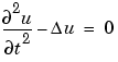
for transverse vibrations of a membrane on a square with corners in (-1,-1), (-1,1), (1,-1), and (1,1). The membrane is fixed (u = 0) at the left and right sides, and is free

at the upper and lower sides. Additionally, we need initial values for

u(t₀) and

The initial values need to match the boundary conditions for the solution to be well-behaved. If we start at t=0,

and

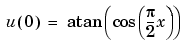
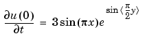
are initial values that satisfy the boundary conditions. The reason for the arctan and exponential functions is to introduce more modes into the solution.

Using the Graphical User Interface

Use the pdetool GUI in the Generic Scalar mode. Draw the square using the Rectangle/square option from the Draw menu or the button with the rectangle icon. Proceed to define the boundary conditions by clicking the button and then double-click the boundaries to define the boundary conditions.

Initialize the mesh by clicking the button or by selecting Initialize mesh from the Mesh menu.

Also, define the hyperbolic PDE by opening the PDE Specification dialog box, selecting the hyperbolic PDE, and entering the appropriate coefficient values. The general hyperbolic PDE is described by

so for the wave equation you get c = 1, a = 0, f = 0, and d = 1.

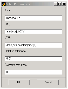
Before solving the PDE, select Parameters . . . from the Solve menu to open the Solve Parameters dialog box. As a list of times, enter linspace(0,5,31) and as initial values for u:

• atan(cos(pi/2*x)) 
  

and for

, enter

• 3*sin(pi*x).*exp(sin(pi/2*y))
  

Finally, click the = button to compute the solution. The best plot for viewing the waves moving in the x and y directions is an animation of the whole sequence of solutions. Animation is a very real time and memory consuming feature, so you may have to cut down on the number of times at which to compute a solution. A good suggestion is to check the Plot in x-y grid option. Using an x-y grid can speed up the animation process significantly.

Using Command-Line Functions

From the command line, solve the equation with the boundary conditions and the initial values above, starting at time 0 and then every 0.05 seconds for five seconds.

The geometry is described in the file squareg.m and the boundary conditions in the file squareb3.m. The following sequence of commands then generates a solution and animates it. First, create a mesh and define the initial values and the times for which you want to solve the equation:

• [p,e,t]=initmesh('squareg'); 
  
  x=p(1,:)'; y=p(2,:)'; 
  
  u0=atan(cos(pi/2*x)); 
  ut0=3*sin(pi*x).*exp(sin(pi/2*y)); 
  
  n=31; 
  tlist=linspace(0,5,n); % list of times 
  

You are now ready to solve the wave equation. The general form for the hyperbolic PDE in the PDE Toolbox is

so here you have d = 1, c = 1, a = 0, and f = 0:

• uu=hyperbolic(u0,ut0,tlist,'squareb3',p,e,t,1,0,0,1); 
  

To visualize the solution, you can animate it. Interpolate to a rectangular grid to speed up the plotting:

• delta=-1:0.1:1; 
  [uxy,tn,a2,a3]=tri2grid(p,t,uu(:,1),delta,delta); 
  gp=[tn;a2;a3]; 
  
  umax=max(max(uu)); 
  umin=min(min(uu)); 
  
  newplot 
  M=moviein(n); 
  for i=1:n,      
  pdeplot(p,e,t,'xydata',uu(:,i),'zdata',uu(:,i),...
  'mesh','off','xygrid','on','gridparam',gp,...
  'colorbar','off','zstyle','continuous');      
  axis([-1 1 -1 1 umin umax]); caxis([umin umax]);      
  M(:,i)=getframe; 
  end 
  movie(M,10); 
  

You can find a complete demo of this problem, including animation, in pdedemo6. If you have lots of memory, you can try increasing n, the number of frames in the movie.

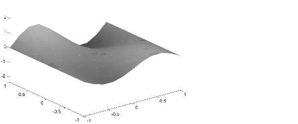
Animation of the Solution to the Wave Equation

Heat Distribution in Radioactive Rod

Examples of Eigenvalue Problems