
| Model Predictive Control Toolbox |   |
Calculates MPC controller gain using a model in MPC step format.
Syntax
Description
Combines the following variables (most of which are optional and have default values) to calculate the MPC gain matrix, Kmpc.
model
is the model of the process to be used in the controller design (in the step format).
The following input variables are optional:
ywt
Is a matrix of weights that will be applied to the setpoint tracking errors. If you use ywt=[ ] or omit it, the default is equal (unity) weighting of all outputs over the entire prediction horizon. If you use ywt, it must have ny columns, where ny is the number of outputs. All weights must be  [ ]
[ ] 0.
0.
You may vary the weights at each step in the prediction horizon by including up to P rows in ywt. Then the first row of ny values applies to the tracking errors in the first step in the prediction horizon, the next row applies to the next step, etc.
If you supply only nrow rows, where 1  nrow <
 P, mpccon will use the last row to fill in any remaining steps. Thus if you wish the weighting to be the same for all P steps, you need only specify a single row.
uwt
Same format as ywt, except that uwt applies to the changes in the manipulated variables. If you use uwt = [ ] or omit it, the default is zero weighting. If uwt  [ ], it must have nu columns, where nu is the number of manipulated variables.
M
There are two ways to specify this variable:
mpccon interprets it as the input horizon (number of moves) as in DMC.
 u = 0 during the optimization and
 cmpc interprets it as a set of nb blocking factors. There may be 1  nb
nb 
P blocking factors, and their sum must be 
P.
If you set M=[ ] or omit it and P , the default is  Inf
InfM=P, which is equivalent to M=ones(1,P). The default value for M is 1 if P=Inf.
P
The number of sampling periods in the prediction horizon. If you set P=Inf or omit it, the default is P=1. If P=inf, the prediction horizon is infinite.
If you take the default values for all the optional variables, you get the "perfect controller," i.e., a model-inverse controller. This controller is not applicable when one or more outputs can not respond to the manipulated variables within one sampling period due to time delay. In this case, the plant-inverse controller is unrealizable. For nonminimum phase discrete plants, this controller is unstable. To counteract this you can penalize changes in the manipulated variables (variable uwt), use blocking (variable M), and/or make P>>M. The model-inverse controller is also relatively sensitive to model error and is best used as a point of reference from which you can progress to a more robust design.
Algorithm
The controller gain is a component of the solution to the optimization problem:

with respect to  (a series of current and future moves in the manipulated variables), where
  (k + j) is a prediction of output i at a time j sampling periods into the future (relative to the current time, k), which is a function of
  , ri(k + j) is the corresponding future setpoint, and nb is the number of blocks or moves of the manipulated variables.
Example
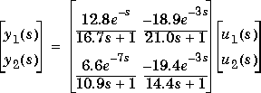
Consider the linear system

:
See the mpccl example for the commands that build the model and a simple controller for this process.
Here is a slightly more complex design with blocking and time-varying weights on the manipulated and output variables:
P=6; M=[2 4];
uwt=[1 0; 0 1];
ywt=[1 0.1; 0.8 0.1; 0.1 0.1];
Kmpc=mpccon(model,ywt,uwt,M,P);
tend=30; r=[1 0];
[y,u]=mpcsim(plant,model,Kmpc,tend,r);
M, above). The uwt selection gives u1 a unity weight and u2 a zero weight for the first move, then switches the weights for the second move. If there had been any additional moves they would have had the same weighting as the second move.
The ywt value assigns a constant weight of 0.1 to y2, and a weight that decreases over the first 3 periods to y1. The weights for periods 4 to 6 are the same as for period 3. The resulting closed-loop (servo) response is:
 | mpccl | mpcinfo |  |