Mapping Toolbox

Terrain

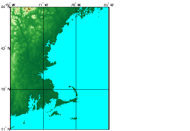
As an example of a higher resolution digital elevation map, MATLAB provides the cape workspace, containing an image of elevation data for the northeastern United States on a 30 arc-second grid (resolution of about one kilometer or better on the ground). The data can be defined as a regular matrix map using the loadcape function script, which rearranges the data and provides the necessary map legend:

• loadcape
  whos
  
  

  Name	Size	Bytes	Class
  caption	2x55	220	char array
  cmap	192x3	4608	double array
  map	360x360	1036800	double array
  maplegend	1x3	24	double array

Here we display the elevation data using a conformal Mercator projection, so shapes of small regions suffer little distortion, while the distortion in relative areas is scarcely noticeable for such a small region.

• axesm('MapProjection','mercator',...
      'MapLatLimit',[41 44],'MapLonLimit',[-72 -69])
  framem
  gridm('MLineLocation',1,'Plinelocation',1,'GLineStyle','-')
  mlabel('MLabelLocation',1)
  plabel('PLabelLocation',1)
  meshm(map,maplegend); demcmap(map)
  

Here is the result:

Global coverage of digital terrain and bathymetry at this resolution is provided through the Mapping Toolbox External Data Interface. A variety of freely available digital elevation maps is available over the Internet for import into MATLAB. These maps range in resolution from about 10 km to 30 meters. See External Data Interface for more information on the data and import functions.

United States Matrix Data

Astronomical Data