Financial Derivatives Toolbox

Pricing and Sensitivity from BDT

This section explains how to use the Financial Derivatives Toolbox to compute prices and sensitivities of several financial instruments using the Black-Derman-Toy (BDT) model. For information, see:

• Pricing and the Price Tree for a discussion of using the bdtprice function to compute prices for a portfolio of instruments.
• Calculating Prices and Sensitivities for a discussion of using the bdtsens function to compute delta, gamma, and vega portfolio sensitivities.

Pricing and the Price Tree

For the BDT model, the function bdtprice calculates the price of any set of supported instruments, based on an interest rate tree. The function is capable of pricing these instrument types:

• Bonds
• Bond options
• Arbitrary cash flows
• Fixed-rate notes
• Floating-rate notes
• Caps
• Floors
• Swaps

The syntax used for calling bdtprice is

• [Price, PriceTree] = bdtprice(BDTTree, InstSet, Options)
  

This function requires two input arguments: the interest rate tree, BDTTree, and the set of instruments, InstSet. An optional argument Options further controls the pricing and the output displayed.

BDTTree is the Black-Derman-Toy tree sampling of an interest rate process, created using bdttree. See Building a BDT Interest Rate Tree to learn how to create this structure based on the volatility model, the interest rate term structure, and the time layout.

InstSet is the set of instruments to be priced. This structure represents the set of instruments to be priced independently using the BDT model. The section Creating and Managing Instrument Portfolios explains how to create this variable.

Options is an options structure created with the function derivset. This structure defines how the BDT tree is used to find the price of instruments in the portfolio, and how much additional information is displayed in the command window when calling the pricing function. If this input argument is not specified in the call to bdtprice, a default Options structure is used.

bdtprice classifies the instruments and calls appropriate pricing function for each of the instrument types. The pricing functions are bondbybdt, cfbybdt, fixedbybdt, floatbybdt, optbndbybdt, and swapbybdt. You can also use these functions directly to calculate the price of sets of instruments of the same type. See the documentation for these individual functions for further information.

BDT Pricing Example

Consider the following example, which uses the data in the MAT-file deriv.mat included in the toolbox. Load the data into the MATLAB workspace.

• load deriv.mat
  

Use the MATLAB whos command to display a list of the variables loaded from the MAT-file.

• whos
  
  Name               Size         Bytes  Class
  
    BDTInstSet         1x1            22708  struct array
    BDTTree            1x1             5522  struct array
    HJMInstSet         1x1            22700  struct array
    HJMTree            1x1             6318  struct array
    ZeroInstSet        1x1            14442  struct array
    ZeroRateSpec       1x1             1580  struct array
  

BDTTree and BDTInstSet are the input arguments needed to call the function bdtprice.

Use the function instdisp to examine the set of instruments contained in the variable BDTInstSet.

• instdisp(BDTInstSet)
  
  
  

  Index Type CouponRate Settle       Maturity     Period Basis .........            Name      Quantity 1     Bond 0.1        01-Jan-2000  01-Jan-2003  1      NaN.........               10% bond  100 2  Bond 0.1        01-Jan-2000  01-Jan-2004  2      NaN.........               10% bond  50 Index Type    UnderInd OptSpec Strike ExerciseDates AmericanOpt Name        Quantity 3 OptBond 1        call    9501   Jan-2002       NaN Option 95   -50 Index Type CouponRate Settle      Maturity       FixedReset Basis Principal Name      Quantity 4     Fixed 0.10       01-Jan-2000 01-Jan-2003 1          NaN NaN 10% Fixed 80 Index Type Spread Settle      Maturity    FloatReset  Basis Principal Name       Quantity 5 Float 20     01-Jan-2000 01-Jan-2003 1           NaN NaN       20BP Float 8 Index Type Strike Settle Maturity CapReset Basis Principal Name  Quantity 6 Cap 0.15   01-Jan-2000 01-Jan-2004 1 NaN NaN 15% Cap 30 Index Type Strike Settle      Maturity       FloorReset Basis Principal Name     Quantity 7 Floor 0.09   01-Jan-2000 01-Jan-2004 1          NaN NaN 9% Floor 40 Index Type LegRate   Settle        Maturity     LegReset Basis Principal LegType Name          Quantity 8 Swap [0.15 10] 01-Jan-2000   01-Jan-2003  [1 1]   NaN NaN [NaN]   15%/10BP Swap 10

Note that there are eight instruments in this portfolio set: two bonds, one bond option, one fixed rate note, one floating rate note, one cap, one floor, and one swap. Each instrument has a corresponding index that identifies the instrument prices in the price vector returned by bdtprice.

Now use bdtprice to calculate the price of each instrument in the instrument set.

• [Price, PriceTree] = bdtprice(BDTTree, BDTInstSet)
  Warning: Not all cash flows are aligned with the tree. Result will 
  be approximated.
  
  Price =
  
     95.5030
     93.9079
      1.7657
     95.5030
    100.6054
      1.4863
      0.0245
      7.3032
  

Note    The warning shown above appears because some of the cash flows for the second bond do not fall exactly on a tree node. This situation is discussed in HJM Pricing Options Structure.

Price Vector

The prices in the vector Price correspond to the prices at observation time zero (tObs = 0), which is defined as the valuation date of the interest rate tree. The instrument indexing within Price is the same as the indexing within InstSet. In this example, the prices in the Price vector correspond to the instruments in the following order.

• InstNames = instget(BDTInstSet, 'FieldName','Name')
  
  InstNames =
  
  10% Bond     
  10% Bond     
  Option 95    
  10% Fixed    
  20BP Float   
  15% Cap      
  9% Floor     
  15%/10BP Swap
  

Consequently, in the Price vector, the fourth element, 95.5030, represents the price of the fourth instrument (10% fixed-rate note); the sixth element, 1.4863, represents the price of the sixth instrument (15% cap).

Price Tree Structure

The output price tree structure PriceTree holds all the pricing information. The first field of this structure, FinObj, indicates that this structure represents a price tree. The second field, PTree is the tree holding the price of the instruments in each node of the tree. The third field, AITree is the tree holding the accrued interest of the instruments in each node of the tree. The fourth field, tObs, represents the observation time of each level of PTree and AITree, with units in terms of compounding periods.

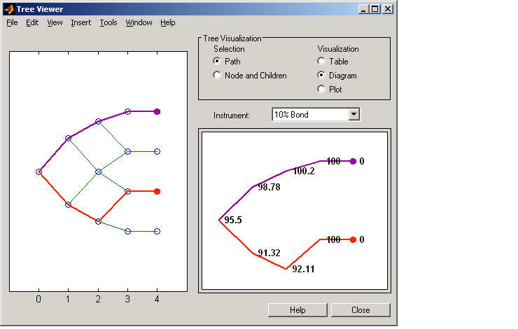
The function treeviewer provides a graphical representation of the tree, allowing you to examine interactively the values on the nodes of the tree.

• treeviewer(PriceTree, BDTInstSet)
  
  
  

Alternatively, you can directly examine the field within the PriceTree structure, which contains the price tree with the price vectors at every state. The first node represents tObs = 0, corresponding to the valuation date.

• PriceTree.PTree{1}
  
  ans =
  
     95.5030
     93.9079
      1.7657
     95.5030
    100.6054
      1.4863
      0.0245
      7.3032
  

You can also use treeviewer instrument-by-instrument to observe instrument prices. For the first 10% bond in the instrument portfolio, treeviewer indicates a valuation date price of 95.5030, the same value obtained by accessing the PriceTree structure directly.

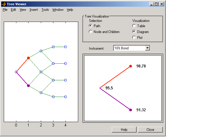
The second node represents the first rate observation time, tObs = 1. This node displays two states, one representing the branch going up and the other one representing the branch going down.

Examine the prices of the node corresponding to the up branch.

• PriceTree.PTree{2}(:,1)
  
  ans =
  
     98.7816
     97.9770
      3.1458
     98.7816
    101.9562
      0.5008
      0.0540
      5.6282
  

As before, you can use treeviewer, this time to examine the price for the 10% bond on the up branch. treeviewer displays a price of 98.7816 for the first node of the up branch, as expected.

Now examine the corresponding down branch.

• PriceTree.PTree{2}(:,2)
  
  ans =
  
     91.3250
     88.1322
      0.7387
     91.3250
     98.9758
      2.7691
          0
      0.6390
  

Use treeviewer once again, now to observe the price of the 10% bond on the down branch. The displayed price of 91.3250 conforms to the price obtained from direct access of the PriceTree structure. You may continue this process as far along the price tree as you want.

Using BDT Trees in MATLAB

BDT Pricing Options Structure