Curve Fitting Toolbox

Custom Equations

If the toolbox library does not contain the desired parametric equation, you must create your own custom equation. However, if possible, you should use the library equations because they offer the best chance for rapid convergence. This is because

• For most models, optimal default coefficient starting points are calculated. For custom equations, the default starting points are chosen at random on the interval [0,1]. Refer to Default Coefficient Parameters for more information.
• An analytic Jacobian is used instead of finite differencing.
• When using the Analysis GUI, analytic derivatives are calculated as well as analytic integrals if the integral can be expressed in closed form.

Note    To save custom equations for later use, you should save the curve-fitting session with the File-> Save Session menu item.

You create custom equations with the Create Custom Equation GUI. The GUI contains two panes: a pane for creating linear equations and a pane for creating general (nonlinear) equations. These panes are described below.

Linear Equations

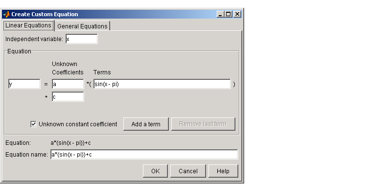
Linear equations are defined as equations that are linear in the parameters. For example, the polynomial library equations are linear. The Linear Equations pane is shown below followed by a description of its parameters.

• Independent variable -- Symbol representing the independent (predictor) variable. The default symbol is x.
• Equation -- Symbol representing the dependent (response) variable followed by the linear equation. The default symbol is y.
• Unknown Coefficients -- The unknown coefficients to be determined by the fit. The default symbols are a, b, c, and so on.
• Terms -- Functions that depend only on the independent variable and constants. Note that if you attempt to define a term that contains a coefficient to be fitted, an error is returned.
• Unknown constant coefficient -- If selected, a constant term is included in the equations to be fit. Otherwise, a constant term is not included.
• Add a term -- Add a term to the equation. An unknown coefficient is automatically added for each new term.
• Remove last term -- Remove the last term added to the equation.
• Equation -- The custom equation.
• Equation name -- The name of the equation. By default, the name is automatically updated to be identical to the custom equation given by Equation. If you override the default, the name is no longer automatically updated.

General Equations

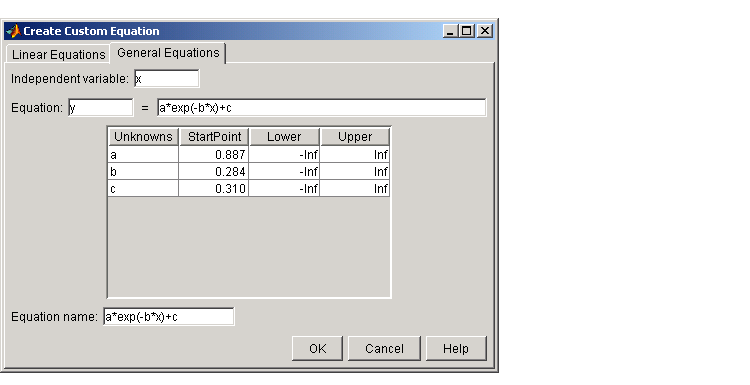
General (nonlinear) equations are defined as equations that are nonlinear in the parameters, or are a combination of linear and nonlinear in the parameters. For example, the exponential library equations are nonlinear. The General Equations pane is shown below followed by a brief description of its parameters.

• Independent variable -- Symbol representing the independent (predictor) variable. The default symbol is x.
• Equation -- Symbol representing the dependent (response) variable followed by the general equation. As you type in the terms of the equation, the unknown coefficients, associated starting values, and constraints automatically populate the table. By default, the starting values are randomly selected on the interval [0,1] and are unconstrained.

• You can immediately change the default starting values and constraints in this table, or you can change them later using the Fit Options GUI.

• Equation name -- The name of the equation. By default, the name is automatically updated to be identical to the custom equation given by Equation. If you override the default, the name is no longer automatically updated.

Note that even if you define a linear equation, a nonlinear fitting procedure is used. Although this is allowed by the toolbox, it is an inefficient process and can result in less than optimal fitted coefficients. Instead, you should use the Linear Equations pane to define the equation.

Library Models

Specifying Fit Options