Using the Symbolic Math Toolbox (Symbolic Math Toolbox)

Symbolic Math Toolbox

Integration

If f is a symbolic expression, then

```
int(f)
```

attempts to find another symbolic expression, F, so that diff(F) = f. That is, int(f) returns the indefinite integral or antiderivative of f (provided one exists in closed form). Similar to differentiation,

```
int(f,v)
```

uses the symbolic object v as the variable of integration, rather than the variable determined by findsym. See how int works by looking at this table.

Mathematical Operation
MATLAB Command

int(x^n) or
int(x^n,x)

int(sin(2*x),0,pi/2) or int(sin(2*x),x,0,pi/2)

g = cos(a*t + b) int(g) or
int(g,t)

int(besselj(1,z)) or
int(besselj(1,z),z)

Mathematical Operation	MATLAB Command
	`int(x^n)` or `int(x^n,x)`
	`int(sin(2x),0,pi/2)` or `int(sin(2x),x,0,pi/2)`
	`g = cos(a*t + b) int(g)` or `int(g,t)`
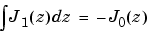	`int(besselj(1,z))` or `int(besselj(1,z),z)`

In contrast to differentiation, symbolic integration is a more complicated task. A number of difficulties can arise in computing the integral. The antiderivative, F, may not exist in closed form; it may define an unfamiliar function; it may exist, but the software can't find the antiderivative; the software could find it on a larger computer, but runs out of time or memory on the available machine. Nevertheless, in many cases, MATLAB can perform symbolic integration successfully. For example, create the symbolic variables

```
syms a b theta x y n x1 u z
```

These tables illustrate integration of expressions containing those variables.

f
int(f)

x^n
x^(n+1)/(n+1)

y^(-1)
log(y)

n^x
1/log(n)*n^x

sin(a*theta+b)
-1/a*cos(a*theta+b)

exp(-x1^2)
1/2*pi^(1/2)*erf(x1)

1/(1+u^2)
atan(u)

f	int(f)
`x^n`	`x^(n+1)/(n+1)`
`y^(-1)`	`log(y)`
`n^x`	`1/log(n)*n^x`
`sin(a*theta+b)`	`-1/acos(atheta+b)`
`exp(-x1^2)`	`1/2pi^(1/2)erf(x1)`
`1/(1+u^2)`	`atan(u)`

The last example shows what happens if the toolbox can't find the antiderivative; it simply returns the command, including the variable of integration, unevaluated.

Definite integration is also possible. The commands

```
int(f,a,b)
```

and

```
int(f,v,a,b)
```

are used to find a symbolic expression for

respectively.

Here are some additional examples.

f
a, b
int(f,a,b)

x^7
0, 1
1/8

1/x
1, 2
log(2)

log(x)*sqrt(x)
0, 1
-4/9

exp(-x^2)
0, inf
1/2*pi^(1/2)

besselj(1,z)
0, 1
1/4*hypergeom([1],[2, 2],-1/4)

f	a, b	int(f,a,b)
`x^7`	`0, 1`	`1/8`
`1/x`	`1, 2`	`log(2)`
`log(x)*sqrt(x)`	`0, 1`	`-4/9`
`exp(-x^2)`	`0, inf`	`1/2*pi^(1/2)`
`besselj(1,z)`	`0, 1`	`1/4*hypergeom([1],[2, 2],-1/4)`

For the Bessel function (besselj) example, it is possible to compute a numerical approximation to the value of the integral, using the double function. The command

```
a = int(besselj(1,z),0,1)
```

returns

```
a =
1/4*hypergeom([1],[2, 2],-1/4)
```

and the command

```
a = double(a)
```

returns

```
a =
  0.2348
```

Integration with Real Constants

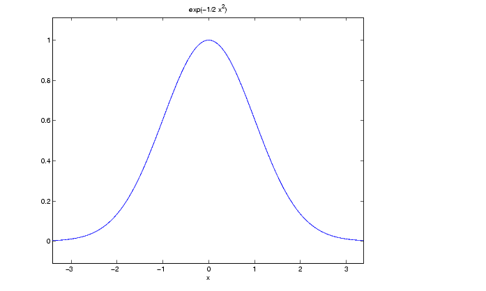
One of the subtleties involved in symbolic integration is the "value" of various parameters. For example, the expression

is the positive, bell shaped curve that tends to 0 as x tends to for any real number k. An example of this curve is depicted below with

and generated, using these commands:

syms x
k = sym(1/sqrt(2));
f = exp(-(k*x)^2);
ezplot(f)

The Maple kernel, however, does not, a priori, treat the expressions or as positive numbers. To the contrary, Maple assumes that the symbolic variables and as a priori indeterminate. That is, they are purely formal variables with no mathematical properties. Consequently, the initial attempt to compute the integral

in the Symbolic Math Toolbox, using the commands

syms x k;
f = exp(-(k*x)^2);
int(f,x,-inf,inf)

results in the output

Definite integration: Can't determine if the integral is 
convergent.
Need to know the sign of --> k^2
Will now try indefinite integration and then take limits.

Warning: Explicit integral could not be found.
ans =
int(exp(-k^2*x^2),x= -inf..inf)

In the next section, you will see how to make a real variable and therefore positive.

Real Variables via sym

Notice that Maple is not able to determine the sign of the expression k^2. How does one surmount this obstacle? The answer is to make k a real variable, using the sym command. One particularly useful feature of sym, namely the real option, allows you to declare k to be a real variable. Consequently, the integral above is computed, in the toolbox, using the sequence

```
syms k real
int(f,x,-inf,inf)
```

which returns

```
ans =
signum(k)/k*pi^(1/2)
```

Notice that k is now a symbolic object in the MATLAB workspace and a real variable in the Maple kernel workspace. By typing

```
clear k
```

you only clear k in the MATLAB workspace. To ensure that k has no formal properties (that is, to ensure k is a purely formal variable), type

```
syms k unreal
```

This variation of the syms command clears k in the Maple workspace. You can also declare a sequence of symbolic variables w, y, x, z to be real, using

```
syms w x y z real
```

In this case, all of the variables in between the words syms and real are assigned the property real. That is, they are real variables in the Maple workspace.

Limits Symbolic Summation