Using the Symbolic Math Toolbox (Symbolic Math Toolbox)

Symbolic Math Toolbox

Eigenvalue Trajectories

This example applies several numeric, symbolic, and graphic techniques to study the behavior of matrix eigenvalues as a parameter in the matrix is varied. This particular setting involves numerical analysis and perturbation theory, but the techniques illustrated are more widely applicable.

In this example, we consider a 3-by-3 matrix A whose eigenvalues are 1, 2, 3. First, we perturb A by another matrix E and parameter . As t increases from 0 to 10^-6, the eigenvalues , , change to , , .

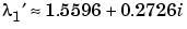This, in turn, means that for some value of , the perturbed matrix has a double eigenvalue .

Let's find the value of t, called , where this happens.

The starting point is a MATLAB test example, known as gallery(3).

A = gallery(3)
A =
  -149      -50     -154
   537      180      546
   -27       -9      -25

This is an example of a matrix whose eigenvalues are sensitive to the effects of roundoff errors introduced during their computation. The actual computed eigenvalues may vary from one machine to another, but on a typical workstation, the statements

```
format long
e = eig(A)
```

produce

e =  
   0.99999999999642   
   2.00000000000579  
   2.99999999999780

Of course, the example was created so that its eigenvalues are actually 1, 2, and 3. Note that three or four digits have been lost to roundoff. This can be easily verified with the toolbox. The statements

B = sym(A);
e = eig(B)'
p = poly(B)
f = factor(p)

produce

e =
[1,  2,  3]

p =
x^3-6*x^2+11*x-6

f =
(x-1)*(x-2)*(x-3)

Are the eigenvalues sensitive to the perturbations caused by roundoff error because they are "close together"? Ordinarily, the values 1, 2, and 3 would be regarded as "well separated." But, in this case, the separation should be viewed on the scale of the original matrix. If A were replaced by A/1000, the eigenvalues, which would be .001, .002, .003, would "seem" to be closer together.

But eigenvalue sensitivity is more subtle than just "closeness." With a carefully chosen perturbation of the matrix, it is possible to make two of its eigenvalues coalesce into an actual double root that is extremely sensitive to roundoff and other errors.

One good perturbation direction can be obtained from the outer product of the left and right eigenvectors associated with the most sensitive eigenvalue. The following statement creates

```
E = [130,-390,0;43,-129,0;133,-399,0]
```

the perturbation matrix

E =
130  -390     0
 43  -129     0
133  -399     0

The perturbation can now be expressed in terms of a single, scalar parameter t. The statements

```
syms x t
A = A+t*E
```

replace A with the symbolic representation of its perturbation:

A = 
[-149+130*t, -50-390*t, -154]
[  537+43*t, 180-129*t,  546]
[ -27+133*t,  -9-399*t,  -25]

Computing the characteristic polynomial of this new A

```
p = poly(A)
```

gives

p =
x^3-6*x^2+11*x-t*x^2+492512*t*x-6-1221271*t

Prettyprinting

```
pretty(collect(p,x))
```

shows more clearly that p is a cubic in x whose coefficients vary linearly with t.

   3              2
  x  + (- t - 6) x  + (492512 t + 11) x - 6 - 1221271 t

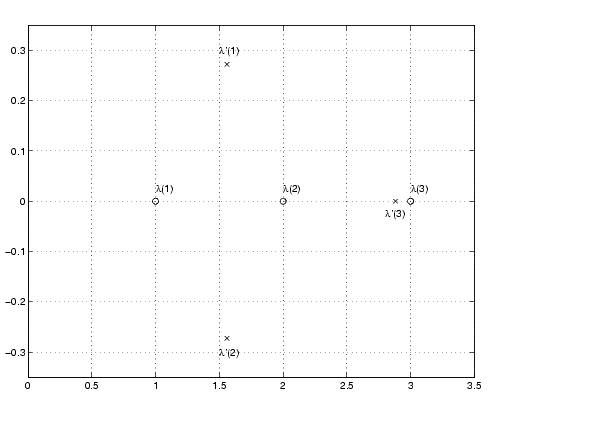
It turns out that when t is varied over a very small interval, from 0 to 1.0e-6, the desired double root appears. This can best be seen graphically. The first figure shows plots of p, considered as a function of x, for three different values of t: t = 0, t = 0.5e-6, and t = 1.0e-6. For each value, the eigenvalues are computed numerically and also plotted:

x = .8:.01:3.2;   
for k = 0:2
  c = sym2poly(subs(p,t,k*0.5e-6));
  y = polyval(c,x);
  lambda = eig(double(subs(A,t,k*0.5e-6)));
  subplot(3,1,3-k)
  plot(x,y,'-',x,0*x,':',lambda,0*lambda,'o')
  axis([.8 3.2 -.5 .5])
  text(2.25,.35,['t = ' num2str( k*0.5e-6 )]);
end

The bottom subplot shows the unperturbed polynomial, with its three roots at 1, 2, and 3. The middle subplot shows the first two roots approaching each other. In the top subplot, these two roots have become complex and only one real root remains.

The next statements compute and display the actual eigenvalues

```
e = eig(A);
pretty(e)
```

showing that e(2) and e(3) form a complex conjugate pair:

[                        1/3                                     ]
[                  1/3 %1    - 3 %2 + 2 + 1/3 t                  ]
[                                                                ]
[        1/3                               1/2        1/3        ]
[- 1/6 %1    + 3/2 %2 + 2 + 1/3 t + 1/2 i 3    (1/3 %1    + 3 %2)]
[                                                                ]
[        1/3                               1/2        1/3        ]
[- 1/6 %1    + 3/2 %2 + 2 + 1/3 t - 1/2 i 3    (1/3 %1    + 3 %2)]
 
                           2    3                     
%1 := 3189393 t - 2216286 t  + t  + 3 (-3 + 4432572 t 
                      2                      3
     - 1052829647418 t + 358392752910068940 t  
                     4 1/2
     - 181922388795 t )
 
                                2
      - 1/3 + 492508/3 t - 1/9 t
%2 := ---------------------------
                   1/3
                 %1

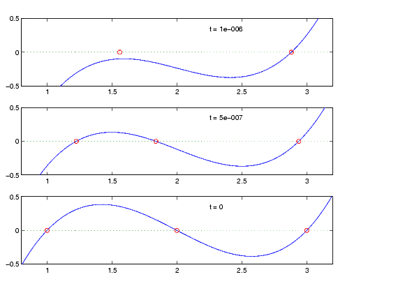
Next, the symbolic representations of the three eigenvalues are evaluated at many values of t

tvals = (2:-.02:0)' * 1.e-6;
r = size(tvals,1);
c = size(e,1);
lambda = zeros(r,c);
for k = 1:c
   lambda(:,k) = double(subs(e(k),t,tvals));
end
plot(lambda,tvals)
xlabel('\lambda'); ylabel('t');
title('Eigenvalue Transition')

to produce a plot of their trajectories.

Above t = 0.8e^-6, the graphs of two of the eigenvalues intersect, while below t = 0.8e^-6, two real roots become a complex conjugate pair. What is the precise value of t that marks this transition? Let denote this value of t.

One way to find the exact value of involves polynomial discriminants. The discriminant of a quadratic polynomial is the familiar quantity under the square root sign in the quadratic formula. When it is negative, the two roots are complex.

There is no discrim function in the toolbox, but there is one in Maple and it can be accessed through the toolbox's maple function. The statement

```
mhelp discrim
```

provides a brief explanation. Use these commands

syms a b c x
maple('discrim', a*x^2+b*x+c, x)

to show the generic quadratic's discriminant, b² - 4ac:

```
ans =
-4*a*c+b^2
```

The discriminant for the perturbed cubic characteristic polynomial is obtained, using

```
discrim = maple('discrim',p,x)
```

which produces

[discrim =
4-5910096*t+1403772863224*t^2-477857003880091920*t^3+2425631850
60*t^4]

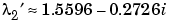
The quantity is one of the four roots of this quartic. Let's find a numeric value for .

digits(24)     
s = solve(discrim);
tau = vpa(s)
tau =
[                        1970031.04061804553618913]
[                                 .783792490602e-6]
[ .1076924816049e-5+.318896441018863170083895e-5*i]
[ .1076924816049e-5-.318896441018863170083895e-5*i]

Of the four solutions, we know that

```
tau = tau(2)
```

is the transition point

```
tau =
.783792490602e-6
```

because it is closest to our previous estimate.

A more generally applicable method for finding is based on the fact that, at a double root, both the function and its derivative must vanish. This results in two polynomial equations to be solved for two unknowns. The statement

```
sol = solve(p,diff(p,'x'))
```

solves the pair of algebraic equations p = 0 and dp/dx = 0 and produces

sol = 
    t: [4x1 sym]
    x: [4x1 sym]

Find now by

```
tau = double(sol.t(2))
```

which reveals that the second element of sol.t is the desired value of :

```
format short
tau =
   7.8379e-07
```

Therefore, the second element of sol.x

```
sigma = double(sol.x(2))
```

is the double eigenvalue

```
sigma =
   1.5476
```

Let's verify that this value of does indeed produce a double eigenvalue at . To achieve this, substitute for t in the perturbed matrix 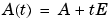and find the eigenvalues of . That is,

e = eig(double(subs(A,t,tau)))
e =
 
   1.5476
   1.5476
   2.9047

confirms that is a double eigenvalue of for t = 7.8379e-07.

Singular Value Decomposition Solving Equations