
| Real-Time Workshop |   |
Look-Up Tables and Polynomials
Simulink provides several blocks that allow approximation of functions. These include blocks that perform direct, interpolated and cubic spline lookup table operations, and a polynomial evaluation block.
There are currently six different blocks in Simulink that perform lookup table operations:
In addition, the Repeating Sequence block uses a lookup table operation, the output of which is a function of the real-time (or simulation-time) clock.
To get the most out of the following discussion, you should familiarize yourself with the features of these blocks, as documented in Using Simulink.
Each type of lookup table block has its own set of options and associated trade-offs. The examples in this section show how to use lookup tables effectively. The techniques demonstrated here will help you achieve maximal performance with minimal code and data sizes.
Multi-Channel Nonlinear Signal Conditioning
Figure 9-6 shows a Simulink model that reads input from two 8-channel, high-speed 8-bit analog/digital converters (ADCs). The ADCs are connected to Type K thermocouples through a gain circuit with an amplification of 250. Since the popular Type K thermocouples are highly nonlinear, there is an international standard for converting their voltages to temperature. In the range of 0 to 500 degrees Celsius, this conversion is a tenth-order polynomial. One way to perform the conversion from ADC readings (0-255) into temperature (in degrees Celsius) is to evaluate this polynomial. In the best case, the polynomial evaluation requires 9 multiplications and 10 additions per channel.
A polynomial evaluation is not the fastest way to convert these 8-bit ADC readings into measured temperature. Instead, the model uses a Direct Look-Up (n-D) Table block (named TypeK_TC) to map 8-bit values to temperature values. This block performs one array reference per channel.
Figure 9-6: Direct Look-Up Table (n-D) Block Conditions ADC Input
The block's table parameter is populated with 256 values that correspond to the temperature at an ADC reading of 0, 1, 2, ... up to 255. The table data, calculated in MATLAB, is stored in the workspace variable TypeK_0_500. The block's Table data parameter field references this variable, as shown in Figure 9-7.
Figure 9-7: Parameters of Direct Look-Up Table (n-D) Block
The model uses a Mux block to collect all similar signals (e.g., Type K thermocouple readings) and feed them into a single Direct Look-Up Table block. This is more efficient than using one Direct Look-Up Table block per device. If multiple blocks share a common parameter (such as the table in this example), Real-Time Workshop creates only one copy of that parameter in the generated code.
This is the recommended approach for signal conditioning when the size of the table can fit within your memory constraints. In this example, the table stores 256 double (8-byte) values, utilizing 2 KB of memory.
Note that the TypeK_TC block processes 16 channels of data sequentially.
Real-Time Workshop generates the following code for the TypeK_TC block shown in Figure 9-6.
/* (LookupNDDirect) Block: <Root>/TypeK_TC */
/* 1-dimensional Direct Look-Up Table returning 16 Scalars */
{
  int_T i1;
  const uint8_T *u0 = &rtb_s1_Data_Type_Conversion[0];
  real_T *y0 = &rtb_root_TypeK_TC[0];

  for (i1=0; i1 < 8; i1++) {
    y0[i1] = (rtP.root_TypeK_TC_table[(uint8_T)u0[i1]]);
  }
  u0 = &rtb_s2_Data_Type_Conversion[0];
  y0 = &rtb_root_TypeK_TC[8];

  for (i1=0; i1 < 8; i1++) {
    y0[i1] = (rtP.root_TypeK_TC_table[(uint8_T)u0[i1]]);
  }
}
Notice that the core of each loop is one line of code that directly retrieves a table element from the table and places it in the block output variable. There are two loops in the generated code because the two simulated ADCs are not merged into a contiguous memory array in the Mux block. Instead, to avoid a copy operation, the Direct Look-Up Table block performs the lookup on two sets of data using a single table array (rtP.root_TypeK_TC_table[]).
If the input accuracy for your application (not to be confused with the number of I/O bits) is 24 bits or less, you can use a single precision table for signal conditioning. Then, cast the lookup table output to double precision for use in the rest of the block diagram. This technique, shown in Figure 9-8, causes no loss of precision.
Figure 9-8: Single Precision Lookup Table Output Is Cast to Double Precision
Note that a direct lookup table covering 24 bits of accuracy would require 64 megabytes of memory, which is typically not practical. To create a single precision table, use the MATLAB single() cast function in your table calculations. Alternatively, you can perform the type cast directly in the Table data parameter, as shown in Figure 9-9.
Figure 9-9: Type Casting Table Data in a Direct Look-Up Block
When table size becomes impractical, you must use other nonlinear techniques, such as interpolation or polynomial techniques. The Look-Up Table (n-D) block supports linear interpolation and cubic spline interpolation.The Polynomial block supports evaluation of noncomplex polynomials.
Compute-Intensive Equations
The blocks described in this section are useful for simplifying fixed, complex relationships that are normally too time consuming to compute in real time.
The only practical way to implement some compute-intensive functions or arbitrary nonlinear relationships in real time is to use some form of lookup table. On processors that do not have floating-point instructions, even functions like sqrt() can become too expensive to evaluate in real time.
An approximation to the nonlinear relationship in a known range will work in most cases. For example, your application might require a square root calculation that your target processor's instruction set does not support. The illustration below shows how you can use a Look-Up Table block to calculate an approximation of the square root function that covers a given range of the function.
The interpolated values are plotted on the block icon.

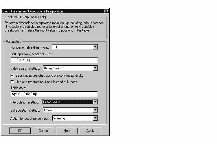
For more accuracy on widely spaced points, use a cubic spline interpolation in the Look-Up Table (n-D) block, as shown below.

Techniques available in Simulink include n-dimensional support for direct lookup, linear interpolations in a table, cubic spline interpolations in a table, and 1-D real polynomial evaluation.
The Look-Up Table (n-D) block supports flat interval lookup, linear interpolation and cubic spline interpolation. Extrapolation for the Look-Up Table (n-D) block can either be disabled (clipping) or enabled for linear or spline extrapolations.
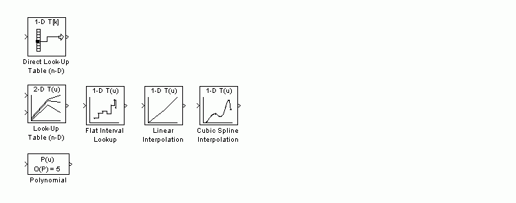
The icons for the Direct Look-Up Table (n-D) and Look-Up Table (n-D) blocks change depending on the type of interpolation selected and the number of dimensions in the table, as illustrated below.

Tables with Repeated Points
The Look-Up Table and Look-Up Table (2-D) blocks, shown below, support linear interpolation with linear extrapolation. In these blocks, the row and column parameters can have repeated points, allowing pure step behavior to be mixed in with the linear interpolations. Note that this capability is not supported by the Look-Up Table (n-D) block.

Slowly vs. Rapidly Changing
Look-Up Table Block Inputs
You can optimize lookup table operations using the Look-Up Table (n-D) block for efficiency if you know the input signal's normal rate of change. Figure 9-10 shows the parameters for the Look-Up Table (n-D) block.
Figure 9-10: Parameter Dialog for the Look-Up Table (n-D) Block
If you do not know the input signal's normal rate of change in advance, it would be better to choose the Binary Search option for the index search in the Look-Up Table (n-D) block and the PreLook-Up Index Search block.
Regardless of signal behavior, if the table's breakpoints are evenly spaced, it is best to select the Evenly Spaced Points option from the Look-Up Table (n-D) block's parameter dialog.
If the breakpoints are not evenly spaced, first decide which of the following best describes the input signal behavior.
Given behavior 1, the best optimization for a given lookup table is to use the Linear search option and Begin index searches using previous index results options, as shown below.
Given behavior 2, the Begin index searches using previous index results option does not necessarily improve performance. Choose the Binary Search option, as shown below.
The choice of an index search method can be more complicated for lookup table operations of two or more dimensions with linear interpolation. In this case, several signals are input to the table. Some inputs may have evenly spaced points, while others may exhibit behavior 1 or behavior 2.
Here it may be best to use PreLook-Up Index Search blocks with different search methods (evenly spaced, linear search or binary search) chosen according to the input signal characteristics. The outputs of these search blocks are then connected to an Interpolation (n-D) Using PreLook-Up Index Search block, as shown in the block diagram below.
You can configure each PreLook-Up Index Search block independently to use the best search algorithm for the breakpoints and input time variation cases.
Multiple Tables with Common Inputs
The index search can be the most time consuming part of flat or linear interpolation calculations. In large block diagrams, lookup table blocks often have the same input values as other lookup table blocks. If this is the case in your block diagram, you can obtain a large savings in computation time by making the breakpoints common to all tables. This savings is obtained by using one set of PreLook-Up Index Search blocks to perform the searches once for all tables, so that only the interpolation remains to be calculated. Figure 9-11 is an example of a block diagram that can be optimized by this method.
Figure 9-11: Before Optimization
Assume that Table A's breakpoints are the same as Table B's first input breakpoints, and that Table C's breakpoints are the same as Table B's second input breakpoints.
A 50% reduction in index search time is obtained by pulling these common breakpoints out into a pair of PreLook-Up Index Search blocks, and using Interpolation (n-D) Using PreLook-Up Index Search blocks to perform the interpolation. Figure 9-12 shows the optimized block diagram.
Figure 9-12: After Optimization
In Figure 9-12, the Look-Up Table (n-D) blocks have been replaced with Interpolation (n-D) Using PreLook-Up blocks.The PreLook-Up Index Search blocks have been added to perform the index searches separately from the interpolations, in order to realize the savings in computation time.
In large controllers and simulations, it is not uncommon for hundreds of multidimensional tables to rely on a dozen or so breakpoint sets. Using the optimization technique shown in this example, you can greatly increase the efficiency of your application.
 | Block Diagram Performance Tuning | Accumulators |  |