| SimPowerSystems | |
Load Flow and Machine Initialization
In order to start the simulation in steady state with sinusoidal currents and constant speeds, all the machine states must be initialized properly. This is a difficult task to perform manually, even for a simple system. In the next section you learn how to use the Load Flow option of the powergui to perform a load flow and initialize the machines.
Double-click the powergui. In the Tools menu, select the Load Flow and Machine Initialization button. A new window appears. In the upper right window you have a list of the machines appearing in your system. Select the SM 3.125 MVA machine. Note that for the Bus Type, you have a menu allowing you to choose either PV Generator or Swing Generator.
For synchronous machines you normally specify the desired terminal voltage and the active power that you want to generate (positive power for generator mode) or absorb (negative power for motor mode). This is possible as long as you have a swing (or slack) bus that generates or absorbs the excess power required to balance the active powers throughout the network.
The swing bus can be either a voltage source or any other synchronous machine. If you do not have any voltage source in your system, you must declare one of the machines as a swing machine. In the next section you will make a load flow with the 25 kV voltage source connected to bus B1 used as a swing bus.
Load Flow Without a Swing Machine
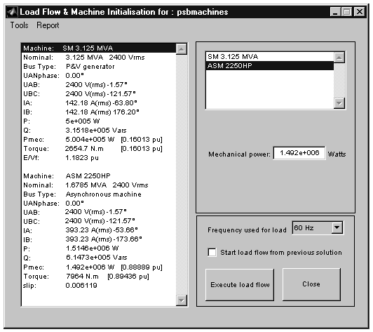
In the Load Flow window, your SM Bus Type should be already initialized as PV generator indicating that the load flow is performed with the machine controlling its active power and terminal voltage. By default, the desired Terminal Voltage is initialized at the nominal machine voltage (2400 Vrms). Keep it unchanged and set the Active Power to 500e3 (500 kW). Now select the ASM 2250 HP machine in the upper right window. The only parameter that is needed is the Mechanical power developed by the motor. Enter 2000*746 (2000 HP). You now perform the load flow with the following parameters.
Select the Execute load flow button. Once the load flow is solved, the phasors of AB and BC machine voltages as well as currents flowing in phases A and B are updated, as shown in the next figure.
The SM active and reactive powers, mechanical power, and field voltage are displayed.
The ASM active and reactive powers absorbed by the motor, slip, and torque are also displayed.
The ASM torque value (7964 N.m) should be already entered in the Constant block connected at the ASM torque input. If you now open the SM and ASM dialog boxes you can see the updated initial conditions. If you open the powergui, you can see updated values of the measurement outputs. You can also click the Nonlinear button to obtain voltages and currents of the nonlinear blocks. For example, you should find that the magnitude of the Phase A voltage across the fault breaker (named Uc_3phase fault/Breaker1) is 20.40 kV, corresponding to a 24.985 kV rms phase-phase voltage.
In order to start the simulation in steady state, the states of the Governor & Diesel Engine and the Excitation blocks should also be initialized according to the values calculated by the load flow. Open the Governor & Diesel Engine subsystem, which is inside the Diesel Engine Speed and Voltage Control subsystem. The initial mechanical power has already been set to 0.1601 p.u. Open the Excitation block and notice that the initial terminal voltage and field voltage have been set respectively to 1.0 and 1.182 p.u.
Note that the load flow automatically initializes the machine blocks but not the associated control blocks. Therefore, if you perform a new load flow, you should change the initial values in the control blocks.
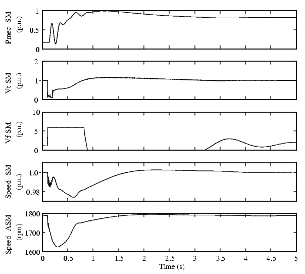
Open the four scopes displaying the terminal voltage, field voltage, mechanical power, and speed of the synchronous machine, as well as the scope displaying the asynchronous motor speed. Start the simulation. The simulation results are shown in the following figure.
Figure 1-22: Simulation Results
Observe that during the fault the terminal voltage drops to about 0.2 p.u. and the excitation voltage hits the limit of 6 p.u. After fault clearing and islanding, the SM mechanical power quickly increases from its initial value of 0.16 p.u. to 1 p.u. and stabilizes at the final value of 0.80 p.u. required by the resistive and motor load (1.0 MW resistive load + 1.51 MW motor load = 2.51 MW = 2.51/3.125 = 0.80 p.u.). After 3 seconds the terminal voltage stabilizes close to its reference value of 1.0 p.u. The motor speed temporarily decreases from 1789 rpm down to 1625 rpm, then recovers close to its normal value after 2 seconds.
If you increase the fault duration to 12 cycles by changing the breaker opening time to 0.3 s, you will notice that the system collapses. The ASM speed slows down to zero after 2 seconds.
Load Flow with a Swing Machine
In this section you make a load flow with two machine types: a PV generator and a Swing generator. In your psbmachines window, delete the inductive source and replace it with the Simplified Synchronous Machine block in p.u. that you find in the Machines library. Rename it SSM 1000MVA and save this new system in your working directory as psbmachine2. Open the SSM 1000MVA dialog box and enter the following parameters.
Second line: Vn(V), Pn(VA) fn(Hz): [1000e6 25e3 60]
Third line: H(s) Kd() p () [inf 0 2]
As you specify an infinite inertia, the speed and therefore the frequency of the machine are kept constant.
Fourth line: R(p.u.) X(p.u.): [0.1 1.0]
(Notice how easily you can specify an inductive short circuit level of 1000 MVA and a quality factor of 10 with the per unit system.)
Fifth line: Leave all initial conditions at 0.
When there is no voltage source imposing a reference angle for voltages, you must choose one of the synchronous machines as a reference. In a load flow program, this reference is called the swing bus. The swing bus absorbs or generates the power needed to balance the active power generated by the other machines and the power dissipated in loads as well as losses in all elements.
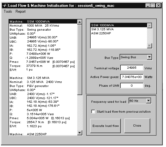
Open the powergui. In the Tools menu, select Load Flow and Machine Initialization. Leave the SM Bus Type as PV Generator and change the SSM Bus Type to Swing Generator. Specify the load flow by entering the following parameters:
For the SSM swing machine you only have to specify the requested terminal voltage (magnitude and phase). The active power is unknown. However, you can specify an active power that is used as an initial guess and help load flow convergence. Specify the following parameters:
SSM: Terminal Voltage = 24985 Vrms(Voltage obtained at bus B1 from the previous load flow);Phase of UAN voltage =0 degrees; Active Power = 0 W
Click the Execute load Flow button. Once the load flow is solved the following solution is displayed. Use the scroll bar of the left window to look at the solution for each of the three machines.
The active and reactive electrical powers, mechanical power, and field voltage are displayed for the SSM block.
The active and reactive electrical powers, mechanical power, and internal voltage of the SM block are
The active and reactive powers absorbed by the motor, slip, and torque of the ASM block are also displayed.
As expected, the solution obtained is exactly the same as the one obtained with the R-L voltage source. The active power delivered by the swing bus is 7.04 MW (6.0 MW resistive load + 1.51 MW load - 0.5 MW generated by SM = 7.01 MW, the difference (0.03 MW) corresponding to losses in the transformer).
Connect at inputs 1 and 2 of the SSM block two Constant blocks specifying respectively the required mechanical power (0.007046 p.u.) and its internal voltage (1.0 p.u.). Restart the simulation. You should get the same waveforms as those of Figure 1-22.
Reference
[1] Yeager, K.E., and J.R.Willis, "Modeling of Emergency Diesel Generators in an 800 Megawatt Nuclear Power Plant," IEEE Transactions on Energy Conversion, Vol. 8, No. 3, September, 1993.
| | Three-Phase Network with Electrical Machines | Session 8: Building and Customizing Nonlinear Models | |