SimPowerSystems

Continuous Variable Time-Step Integration Algorithms

Open the PI section Line dialog box and make sure the number of sections is set to 1. Open the Simulation --> Simulation parameters dialog. As you now have a system containing switches, you need a stiff integration algorithm to simulate the circuit. In the Solver pane, select the variable-step, stiff integration algorithm ode23tb.

Keep the default parameters (relative tolerance set at 1e-3) and set the stop time to 0.02 seconds. Open the scopes and start the simulation. Look at the waveforms of the sending and receiving end voltages on ScopeU1 and ScopeU2.

Once the simulation is complete, copy the variable U2 into U2_1 by entering the following command in the MATLAB window:

• U2_1=U2;
  

These two variables now contain the waveform obtained with a single PI section line model.

Open the PI section Line dialog box and change the number of sections from 1 to 10. Start the simulation. Once the simulation is complete, copy the variable U2 into U2_10.

Before modifying your circuit to use a distributed parameter line model, save your system as circuit2_10pi. You will have to reuse this circuit later.

Delete the PI section line model and replace it with a single phase Distributed Parameter Line block. Set the number of phases to 1 and use the same R, L, C, and length parameters as for the PI section line (see Figure 1-1). Save this system as circuit2_dist.

Restart the simulation and save the U2 voltage in the U2_d variable.

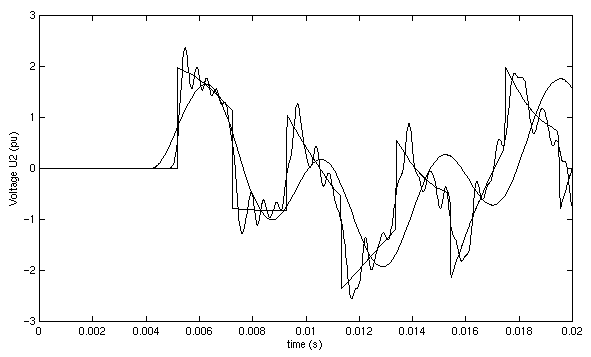
You can now compare the three waveforms obtained with the three line models. Each variable U2_1, U2_10, and U2_d is a two-column matrix where the time is in column 1 and the voltage is in column 2. Plot the three waveforms on the same graph by entering the following command:

• plot(U2_1(:,1), U2_1(:,2), U2_10(:,1),U2_10(:,2),
  U2_d(:,1),U2_d(:,2));
  

These waveforms are shown in the next figure. As expected from the frequency analysis performed during Session 2, the single PI model does not respond to frequencies higher than 229 Hz. The 10 PI section model gives a better accuracy, although high-frequency oscillations are introduced by the discretization of the line. You can clearly see in the figure the propagation time delay of 1.03 ms associated with the distributed parameter line.

Figure 1-6: Receiving End Voltage Obtained with Three Different Line Models

Session 3: Simulating Transients

Discretizing the Electrical System