Nonlinear Control Design Blockset

Case Studies

To provide extended examples of use, this chapter presents four benchmark problems, which are contained separately in the Simulink systems ncddemo1, ncddemo2, ncddemo3, and ncddemo4. All four are contained in the Simulink system ncddemo. The problems increase in sophistication from ncddemo1 to ncddemo4.

Case Study 1: PID Controller

Case Study 2: LQR with Feedforward Controller

Case Study 3: MIMO PI Controller

Case Study 4: Inverted Pendulum on Track

Case Study 1: PID Controller

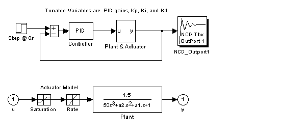
In the first control design problem, ncddemo1, we model the nominal plant as the third-order SISO transfer function.

where a2 = 43 and a1 = 3 nominally with rate limit (±0.8) and saturation (±2) nonlinearities. Additionally, because of design tolerances, actual plant dynamics exhibit significant variation from the nominal. Specifically, the denominator coefficient a2 varies between 40 and 50 and the coefficient a1 varies between one-half and 1.5 time its nominal value of 3.

Problem Definition

We want to design a PID controller for the system so that the closed loop system meets the following tracking specifications:

Maximum overshoot of 20%
Maximum 10 seconds rise time
Maximum 30 seconds settling time

Further, we want the closed loop response to be robust to the uncertainty in the plant dynamics.

Problem Setup

The Simulink system ncddemo1 contains the plant and control structure as shown below. To open the system, type ncddemo1 at the MATLAB prompt or double-click on the Nonlinear Control Design Blockset Demo 1 block in the Simulink system ncddemo. Notice the rate and saturation nonlinearities included in the plant model. A step input drives the system. The NCD block attaches to the plant output since it is the signal to be constrained. Inspecting the System's Parameters dialog box shows that each simulation lasts 100 seconds.

Double-click on the block ncd1init to initialize the tunable and uncertain variables. The uncertain variables, a2 and a1, are initialized to their nominal values of 40 and 3 respectively. The tunable parameters, Kp, Ki, and Kd initialize to 0.63, 0.0504, and 1.9688 respectively. These values result from using the Ziegler-Nichols method for tuning PID controllers [1, Ch.3]. The Ziegler-Nichols method for tuning PID controllers can be summarized as follows:

Set the integral and derivative gains to zero and increase the proportional gain until the system just becomes unstable.
Define this gain to be Ku and measure the period of oscillation, Pu.
Set Kp = 3*Ku/5, Ki = 6*Ku/(5*Pu), and Kd = 3*Ku*Pu/40.

Double-clicking on the ncd1init block also defines the time domain response constraints for this demonstration. Double-click on the NCD block to open the Nonlinear Control Design Blockset constraint figure and display the constraints. The lower and upper constraint bounds effectively define overshoot, rise time, and settling time constraints.

Problem Solution

Before starting the optimization, open the Optimization Parameters dialog box by selecting Parameters... from the Optimization menu and notice how the Tunable Variables are defined. Also open the Uncertain Variables dialog box by selecting Uncertainty... from the Optimization menu. Notice how the uncertainty in the parameters a2 and a1 is defined and also note that the optimization constrains only the nominal plant.

Press the Start button, select Start from the Optimization menu, or hold down the accelerator key and press t to start the optimization. Watch the response evolve and improve during the optimization. The optimization time, cost function evolution, and final values for the tunable variables may differ for different computers. However, the optimization should produce a controller that meets all the constraints.

Now return to the Uncertain Variables dialog box and constrain the upper and lower bound plants. Press Start to begin optimizing with uncertainty. You may find that all the constraints cannot now be met, but the displayed output shows a maximum constraint violation of less than 0.01. Considering the degree of uncertainty in the plant dynamics, such a result is still impressive.

You can experiment if you want, moving the constraint bounds in an attempt to achieve even better system performance. For example, decrease the rise time or lower the overshoot constraints.

Case Study 2: LQR with Feedforward Controller

The second problem, ncddemo2, requires the Control System Toolbox as it is an extension of problems found in the Simulink demo file lqgdemos. We model the SISO plant as a fourth-order linear state-space system augmented with saturation (±5) and rate limit (±10) nonlinearities. The equations

define the nominal plant. For illustration purposes, we allow the plant A matrix to vary between one half and twice its nominal value.

Problem Definition

Using LQG/LTR techniques, we design a Kalman state estimator and regulator gain (K) for the linear system. Next we add an integrator to guarantee zero steady state error. To achieve increased response time, we add a feedforward gain (FF). In the Simulink demo system lqgopt, the control parameters K and FF are tuned via a least squares method. We tune these parameters here using the Nonlinear Control Design Blockset.

Specifically, we want to tune the control parameters K and FF such that the closed loop system meets the following tracking specifications:

Maximum overshoot of 20%
Maximum one second rise time
Maximum three second settling time

Further, we want the closed loop response to be robust to the uncertainty in the plant dynamics.

Problem Setup

The Simulink system ncddemo2 contains the plant and control structure shown below. To open the system, type ncddemo2 at the MATLAB prompt or double-click on the Nonlinear Control Design Blockset Demo 2 block in the Simulink system ncddemo. Notice the rate limit (±10) and saturation (±5) nonlinearities included in the plant model. Using the From Workspace block, we input a step that transitions from zero to one at one second. The NCD block attaches to the plant output since it is the signal to be constrained. Inspecting the System's Parameters dialog box shows that each simulation lasts 10 seconds.

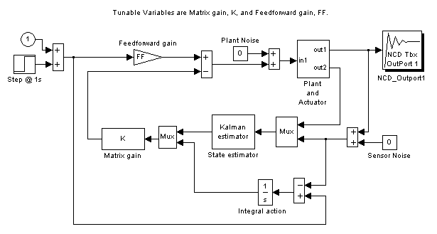
Double-click on the block ncd2init to initialize the tunable and uncertain variables. Double-clicking on the ncd2init block also defines the time domain response constraints for this demonstration. Double-click on the NCD block to open the Nonlinear Control Design Blockset constraint figure and display the constraints. The constraint bounds effectively define overshoot, rise time, and settling time constraints.

As described above, we generate an initial controller design via LQG/LTR methods using the linearized plant. For the present nonlinear control optimization, only the feedforward gain FF and the regulator matrix gain K are tunable.

Problem Solution

Before starting the optimization, open the Optimization Parameters dialog box by selecting Parameters ... from the Optimization menu and notice how the Optimization Parameters are defined. Also open the Uncertain Variables dialog box by selecting Uncertainty ... from the Optimization menu. Notice how the uncertainty in the plant A matrix is defined and also note that the optimization only constrains the nominal plant.

You can experiment if you want, moving the constraint bounds in an attempt to achieve even better system performance. For example, decrease the rise time or lower the overshoot constraints.

Case Study 3: MIMO PI Controller

The third control design problem, ncddemo3, considers designing a MIMO centralized PI controller for the LV100 gas turbine engine. We model the plant as a two-input, two-output, five-state minimum phase system. The inputs are the fuel flow and variable area turbine nozzle. The outputs are the gas generator spool speed and temperature. The five states are the gas generator spool speed, the power output, temperature, fuel flow actuator level, and variable area turbine nozzle actuator level. A state-space model for the system is given by

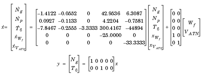
So that comparison can be made to previous results, no nonlinearities are modeled in this problem. As mentioned in [2], saturation nonlinearities do exist in the system in the form of limited actuator effort and maximum temperatures. These nonlinearities could be included in Nonlinear Control Design Blockset problem formulation as in previous examples. Also, for the sake of demonstration, we exaggerate plant uncertainty. Specifically, we allow the plant A matrix to vary between one-half and twice its nominal value.

Problem Definition

We want to design a centralized 2-by-2 PI controller for the plant so that the closed loop system meets the following tracking specifications:

Maximum one second rise time
Zero overshoot in the first channel and less than 10% in the second
Maximum three second settling time
Less than 5% cross channel coupling

Further, we want the closed loop response to be robust to the uncertainty in the plant dynamics.

Problem Setup

The Simulink system ncddemo3 contains the plant and control structure. To open the system, type ncddemo3 at the MATLAB prompt or double-click on the ncddemo3 block in the Simulink system ncddemo. We model the PI controller as a state-space system with a zero A matrix and identity B matrix. The C and D matrices are the tunable variables Ki and Kp respectively for a total of eight tunable variables. Initial values for the controller are generated as in [2].

Double-click on the ncd3init block to load the plant data, signal inputs, initial values for the tunable variables, and previous controller solutions obtained via other methods. Double-clicking on the ncd3init block also defines the time domain response constraints for this demonstration. Notice there are now two Nonlinear Control Design Blockset optimization blocks that can be displayed simultaneously.

The approach we suggest for MIMO controller design for tracking problems involves sequentially stepping the commanded inputs. When the first channel steps, the first output should track the step and the other channels should reject the signal. When the second channel steps, the second output should track the step and the other channels should reject the signal, etc. Notice we have used the From Workspace block to inject such sequentially stepping signals to the system.

Double-click on the NCD blocks to open the Nonlinear Control Design Blockset constraint figures and display the constraints. Notice the constraints for the first output initially define step response bounds as in previous examples (i.e., the first channel is stepped first). Meanwhile the second ouput's constraint bounds merely constrain the signal to stay within ±0.05 of zero. Similarly, when the second channel is stepped, the constraints for the first output merely constrain that signal to within ±0.05 of zero while the second output's constraint bounds appear in the familiar step response configuration.

Problem Solution

Press the Start button, select Start from the Optimization menu, or hold down the accelerator key and press t to start the optimization. Watch the responses evolve and improve during the optimization. The optimization time, cost function evolution, and final values for the tunable variables may be different for different computers. However, the optimization should produce a controller that meets all the constraints.

Case Study 4: Inverted Pendulum on Track

The fourth problem, ncddemo4, considers a variation of the popular inverted pendulum example. Specifically, we attach a cylindrical metal rod to a motor driven cart in such a way as to allow for rotation about only one axis. The cart is mounted on a linear track so as to create a stabilizable problem as shown below.

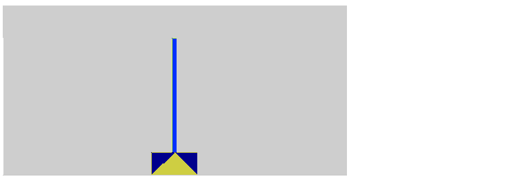
The Appendix provides an explanation of the equations of motion for the cart and pendulum. Besides the inherent nonlinearities of the system equations, limits on the voltage applied to the motor result in an actuation saturation constraint of 1N. Sensors provide cart position and pendulum angle measurements.

Problem Definition

In addition to stabilizing the inverted pendulum, we want the cart to follow a commanded reference signal. Specifically, we want to design a controller for the system to meet the following closed loop tracking specifications when the system is excited with a unit step:

Maximum four seconds rise time
Maximum six seconds settling time
Zero overshoot
Less than 0.2 radian deviation from vertical

Further, we want the closed loop response to be robust to the uncertainty in the plant dynamics. The Appendix explains how to generate an initial stabilizing controller using a linear approximation of the system. We leave it to you to introduce uncertainty (into the pendulum length, cart mass, etc.) if you want. For example, you might explore whether it is more difficult to control the pendulum when it is 50% longer or when it is 50% shorter.

Problem Setup

The Simulink system ncddemo4 contains the plant and control structure. To open the system, type ncddemo4 at the MATLAB prompt or double-click on the Nonlinear Control Design Blockset Demo 4 block in the Simulink system ncddemo. Notice the saturation nonlinearities included in the plant model and the masked pendulum block contain the nonlinear equations of motion for the system. We command the cart position with a unit step input. NCD blocks attach to the pendulum angle and cart position signals. Inspecting the System's Parameters dialog box shows that each simulation lasts 15 seconds.

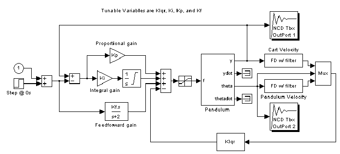
The control structure contains finite difference state estimators for the cart velocity and pendulum angular velocity (i.e., we only have position feedback). As part of an inner control loop (used to stabilize the pendulum), the cart velocity estimate, pendulum angle, and angular velocity estimate are multiplied by a gain, summed, and then input to the motor. We initialize this 1-by-3 gain as Klqr = Clqr(2:4) where Clqr is the 1-by-4 LQR solution described in the Appendix. In an outer control loop (used to allow the cart to follow a commanded signal), a feedforward gain, Kf, is initialized as
Kf = Clqr(1), and an intergral gain, Ki, is initialized to zero. Note that in the absence of a commanded signal, these initial controller values reduce the control structure to the LQR gain described in the previous section.

Double-click on the block ncd4init to initialize the tunable variables as described above and define time domain response constraints for this demonstration. Double-click on the NCD blocks to open the Nonlinear Control Design Blockset constraint figures and display the constraints. By now, the configuration of the cart position constraints should be familiar to you as typical for a step response. Meanwhile the pendulum angle channel contains constraints that essentially define a disturbance rejection problem. In other words, while the cart is moving to its commanded position on the track, the pendulum should remain more-or-less balanced.

Problem Solution

You may notice this optimization runs slower than the other examples. This occurs because the finite state estimators require frequent updating during simulation.

References for Case Studies

[1] Franklin, Gene F., J. David Powell, and Abbas Emami-Naeini, Feedback Control of Dynamic Systems, Addison-Wesley Publishing Company, 1987.

[2] Potvin, A.F. A Unified Solution to Constrained Configuration Control Law Design, Master's Thesis, MIT EECS Dept., 1991.

Strong Stabilization Troubleshooting