Mu Analysis and Synthesis Toolbox

Compute the time response of linear system

Syntax

• y = trsp(sys,u,tfinal,int,x0) 
  y = dtrsp(dsys,u,T,tfinal,x0) 
  [output,y,u] = sdtrsp(sys,k,input,T,tfinal,int,x0,z0)
  

Description
trsp computes the time response of the continuous-time system, sys, with the input, u. The input, u, is a VARYING matrix, which contains the input signal vector at certain points in time. The input can be irregularly spaced in the independent variable or a constant, in which case it is assumed to occur at t = 0.

The final time, tfinal, is an optional argument. If omitted, it defaults to the maximum time in u. The time response is calculated as though the input is a constant value between the points specified in u. If tfinal is greater than the largest independent variable in u, the input is held at the last value in u.

For continuous-time evaluation (trsp), you can optionally specify an integration time with the variable int. If this is omitted, or is equal to zero, an appropriate value is calculated and displayed. The calculated integration time depends on the minimum spacing in the input and the fastest dynamics in sys. int will also be the independent variable step size in the regularly spaced output, y. If a coarser output is adequate, it can be obtained with the function vdcmate.

Initial conditions can optionally be specified with the argument, x0. This specifies the state vector at the first time point in the input vector. If x0 is omitted, or is a zero scalar, then it is assumed to be a zero vector.

trsp interpolates the input with a zero-order hold of step size equal to int, discretizes the output at this same step size, and calculates the response from the initial time to tfinal in steps of int.

dtrsp calculates the response for a discrete-time system, dsys. The time (for the independent variable) between discrete indices is T. If the input is not regularly spaced at intervals of time T, it is interpolated. tfinal and x0 behave in the same manner as for trsp.

sdtrsp calculates a sampled-data time response for a closed-loop system with a continuous generalized plant (sys) and a discrete controller (K). The interconnection is illustrated below.

The signals, output, y, and u are calculated. T is the sampled-data controller sample time, and you have the same input and tfinal options as the trsp function. Similarly, an integration step size, int, can optionally be specified for the continous part of the simulation. Initial conditions can be specified for sys (x0) and K (z0).

Examples
A simple SISO system illustrates the use of trsp. This example shows the consequences of the input being assumed to be constant between time points.

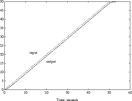
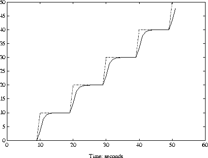
• sys = pck(-1,1,1); 
  minfo(sys)
  system:1 states1 outputs1 inputs
  u = vpck([0:10:50]',[0:10:50]'); 
  y = trsp(sys,u,60);
  integration step size: 0.1
  interpolating input vector (zero order hold)
  minfo(y)
  varying:601 pts1 rows1 cols
  vplot(u,'-.',y,'-') 
  xlabel('time: seconds') 
  text(10,20,'input') 
  text(25,10,'output')
  
  
  

At first glance the output does not seem to be consistent with the plotted input. Remember that trsp assumes that the input is held constant between specified values. The vplot and plot commands display a linear interpolation between points. This can be more clearly seen by displaying the input signal interpolated to at least as small a step size as the default integration step (here 0.1 seconds).

• vplot(u,'-.',vinterp(u,0.1),'--',y,'-') 
  xlabel('time: seconds') 
  text(5,44,'dash-dot: input') 
  text(5,40,'dashed: interpolated input') 
  text(5,36,'solid: output')
  
  
  

• uramp = vinterp(u,0.1,60,1); 
  minfo(uramp)
  varying:601 pts1 rows1 cols
  yramp = trsp(sys,uramp);
  integration step size: 0.1
  vplot(uramp,'-.',yramp,'-') 
  xlabel('time: seconds') 
  text(20,15,'output') 
  text(12,20,'input')
  

Note that because the input is regularly spaced, with spacing less than or equal to the default integration time, the input is not interpolated by trsp. Since no final time was specified in the trsp argument list, and 60 seconds was specified to vinterp as the final time, this becomes the last time in the input vector uramp.

To illustrate the use of dtrsp, a bilinear transformation generates a digital system. The sample time is chosen as 1 second. The output is plotted against a 1 second interpolation of the input.

• T = 1; 
  dsys = tustin(sys,T); 
  ydig = dtrsp(dsys,u,T); 
  vplot(ydig,'-',vinterp(u,1),'-.') 
  xlabel('time: seconds')
  

To illustrate the use of sdtrsp, consider the application of a discrete controller to a double integrator. A continuous plant and a discrete controller are created. A sample and hold equivalent of the plant is formed and the discrete closed-loop system is calculated. Simulating this with dtrsp gives the system response at the sample points. sdtrsp is then used to calculate the intersample behavior.

• P = nd2sys(1,[1,0,0]); 
  T = 1.0/20; 
  C=pck([-1.5 T/4; -2/T -.5],[ .5 2;1/T 1/T], ... 
      [-1/T2 -1.5/T], [1/T2 0]);
  

• Pd = samhld(P,T); 
  systemnames = 'Pd C'; 
  inputvar = '[ref]'; 
  outputvar = '[Pd]'; 
  input_to_Pd = '[C]'; 
  input_to_C = '[ref ; Pd]'; 
  sysoutname = 'dclp'; 
  cleanupsysic = 'yes'; 
  sysic;
  

• ustep = step_tr(0,1,T,20*T); 
  y = dtrsp(dclp,ustep,T);
  

• M = mmult([0,1;1,0;0,1],daug(1,P)); 
  y1 = sdtrsp(M,C,ustep,T); 
  vplot(y,'*',y1,'-') 
  axis([0,1,0,1.5]) 
  xlabel('Time: seconds') 
  title('Step response: discrete (*), &continuous')
  
  
  

Now we look at the effect of a nonzero initial condition in the continuous system. Note how examining the system at only the sample points will underestimate the amplitude of the overshoot.

• y2 = sdtrsp(M,C,vpck(1,0),T,1,0,[1;0]); 
  vplot(y1,'--',y2,'-') 
  axis([0,1,0,1.5]) 
  xlabel('Time: seconds') 
  title('Step response: non zero initial condition')
  
  
  

• M2 = mmult([0,1,1;1,0,0;0,1,1],daug(1,1,P)); 
  dist = sin_tr(41,0.1,0.001,1); 
  [dat,datptr,t] = vunpck(dist); 
  input = abv(vpck(ones(t),t),dist); 
  [y3,meas,act] = sdtrsp(M2,C,input,T); 
  vplot(y3,'-',input,'--') 
  xlabel('Time: seconds') 
  title('Step response: disturbance (dashed) & output (solid)')
  
  
  

Algorithm
trsp first calculates an integration time (or uses the specified integration time) to determine the sample time at which to discretize the continuous-time system. The integration time is taken to be the inverse of 10 times the fastest mode of the input system. The input vector is interpolated at each sample time via a zero-order hold, and then a sample-hold of the input continous system is performed. Finally the time response of the system is performed via a for loop at each integration time step. dtrsp is provided a discrete time system and a sample time. dtrsp first interpolates the input vector via a zero-order hold and then determines the time response via a for loop at each sample time.

Caution:
Systems with fast dynamics lead to very small integration times. This is both time consuming and requires a significant amount of storage. We recommend you residualize the fastest modes of the system, which does not affect the time response. This can be done with the µ-Tools command sresid.

See Also
cos_tr, siggen, sin_tr, step_tr, sysbal, vdcmate, vinterp

szeros

tustin