musynfit, musynflp, muftbtch (Mu Analysis and Synthesis Toolbox)

Mu Analysis and Synthesis Toolbox

musynfit, musynflp, muftbtch

Interactive D-scaling rational fit routines used in old µ-synthesis routines

Note: These routines are included only for backwards compatibility with versions 1.0 and 2.0. They will not be supported in future versions. They should not be used by new users of the toolbox. All new routines should be based on the new routine, msf, which is described on page ???.

Syntax

[dsysL,dsysR] = musynfit(pre_dsysL,dvec,sens,blk,...
                       nmeas,ncntrl,clpg,upbd,wt) 
[dsysL,dsysR] = musynflp(pre_dsysL,dvec,sens,blk,...
                       nmeas,ncntrl,clpg,upbd,wt) 
[dsysL,dsysR] = muftbtch(pre_dsysL,dvec,sens,blk,... 
                       nmeas,ncntrl,dim)

Description
musynfit fits the magnitude curve obtained by multiplying the old D frequency response (from pre_dsysl) with the dvec data. musynfit returns stable, minimum phase system matrices dsysL and dsysR, which can be absorbed into the original interconnection structure. Once absorbed, a H design is performed with hinfsyn completing another D-K iteration of µ-synthesis.

For the first µ-synthesis iteration, set the variable pre_dsysl to the string first. In subsequent iterations, pre_dsysl should be the previous (left) rational D-scaling system matrix, dsysL. Essentially, the element-by-element magnitudes of the matrices mmult(unwrapd(dvec,blk),frsp(pre_dsysL,getiv(dvec))), and frsp(dsysL,getiv(dvec)) are equal.

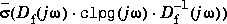
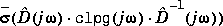
The (optional) variable clpg is the VARYING matrix that produced the dvec, sens, and upbd data output from µ. The fitting procedure is interactive (musynfit or musynflp), and fits (in magnitude) these scalings with rational, stable transfer function matrices, . After fitting the dvec data, plots of

and

are shown in the lower graph window for comparison. At this point, you have the option of refitting the D data. If clpg and upbd are not provided, the default is to plot the sens variable in the the lower graph.

Note:
You are strongly discouraged from calling musynfit and musynflp directly and are encouraged to use dkit or dkitgui to perform µ-synthesis calculations.

Input arguments:

pre_dsysl
is set to the character string 'first' for the first iteration. As the iteration proceeds, it should be the previous dsysL.

sens
is the sensitivity of the upper bound in the µ calculation on the Ds. The sensitivity sens is a frequency domain weight, which is obtained from mu.

dvec
is a frequency varying row vector containing the Ds (from mu).

blk
is the block structure, same block structure used in mu.

nmeas
is the number of measurements in control problem.

ncntrl
is the number of controls in control problem.

clpg
is the frequency response upon which the calculation was performed (optional).

upbd
is the upper bound from the µ calculation (optional).

wt
is a weight used to influence the frequency range in which the data is to be fit more accurately (optional).

dim
is the highest order fit to be used (only used in muftbtch).

`pre_dsysl`	is set to the character string `'first'` for the first iteration. As the iteration proceeds, it should be the previous `dsysL`.
`sens`	is the sensitivity of the upper bound in the µ calculation on the Ds. The sensitivity `sens` is a frequency domain weight, which is obtained from `mu`.
`dvec`	is a frequency varying row vector containing the Ds (from `mu`).
`blk`	is the block structure, same block structure used in `mu`.
`nmeas`	is the number of measurements in control problem.
`ncntrl`	is the number of controls in control problem.
`clpg`	is the frequency response upon which the calculation was performed (optional).
`upbd`	is the upper bound from the µ calculation (optional).
`wt`	is a weight used to influence the frequency range in which the data is to be fit more accurately (optional).
`dim`	is the highest order fit to be used (only used in `muftbtch`).

Output arguments:

dsysL
is the output (left) block diagonal, SYSTEM scaling.

dsysR
is the input (right) block diagonal, SYSTEM scaling (needs to be inverted before being absorbed into the interconnection structure).

musynflp
has the same inputs and outputs and user interaction as musynfit but uses a linear programing routine to do the fitting. muftbtch is a batch version of musynflp that has no user interaction. The extra argument dim is a required argument of parameters for the linear program. dim has the form [hmax htol nmin nmax] where
hmax is a measure of the allowable error in the fit.
htol is a measure of the accuracy with which the optimization is carried out.
nmin and nmax are the minimum and maximum orders considered in the problem

`dsysL`	is the output (left) block diagonal, SYSTEM scaling.
`dsysR`	is the input (right) block diagonal, SYSTEM scaling (needs to be inverted before being absorbed into the interconnection structure).
`musynflp`	has the same inputs and outputs and user interaction as `musynfit` but uses a linear programing routine to do the fitting. `muftbtch` is a batch version of `musynflp` that has no user interaction. The extra argument `dim` is a required argument of parameters for the linear program. `dim` has the form `[hmax htol nmin nmax]` where `hmax` is a measure of the allowable error in the fit. `htol` is a measure of the accuracy with which the optimization is carried `out`. `nmin` and `nmax` are the minimum and maximum orders considered in the problem

For more detail about the role of hmax and htol, see the reference pages for fitmaglp and magfit. Reasonable choices are hmax = .26 and htol = .1.

The musynflp and musynfit commands provide the option of fitting the frequency varying D-scale data by hand using the µ-Tools drawmag command. You can invoke this option with the string 'drawmag' in response to the prompt

```
ENTER ORDER OF CURVE FIT or 'drawmag'
```

The mouse is used in the plot window to identify the data to be fit with a stable, minimum-phase system. See the drawmag command for more information.

Examples
musynfit is used within a D-K iteration (µ-synthesis) to fit the D-scales, which are output from the mu command. The first step in the D-Kiteration is to design an H control law. The closed-loop system is analyzed with mu based on the block structure blk defined. The optimal D-scaling output from mu, which are real coeeficients, are fit with real, rational, minimum-phase stable transfer functions via musynfit. These fitted D-scales are wrapped back around the orginal interconnection structure P. After absorbing the D-scales, another D-K iteration is performed, starting with the design of an H control law for the modified plant. This process usually continues until the value of µ doesn't change significantly between control design iterations.

This example is taken from the "HIMAT Robust Performance Design Example" section in Chapter 7. himat_ic contains the open-loop interconnection structure. It has one multiplicative input perturbation, which is two by two, and has two error signals, and two external disturbances. There are two measurements, and two control inputs to the system. The block structure for the µ-analysis problem is given by blk=[2 2; 2 2].

First step in a D-K iteration is to design an H controller and analyze the closed loop system with µ.

mkhic  
omega = logspace(0,4,40); 
blk = [2 2; 2 2]; 
[k1,g1,gf1] = hinfsyn(himat_ic,2,2,0.8,6,0.05,2); 
g1_g = frsp(g1,omega); 
[bnds1,dvec1,sens1,rp1] = mu(g1_g,blk);

The D-scalings output from the µ-analysis problem needs to be fit with real, rational, stable, minimum-phase transfer functions. This is done with musynfit. The first D-scale is fit with both a first and third-order transfer function, with the third order transfer function selected.

[dsysL1,dsysR1] = musynfit('first',dvec1,sens1,blk,2,2);



ENTER ORDER OF CURVE FIT or 'drawmag' 1



ENTER ORDER OF CURVE FIT or 'drawmag' 3



ENTER ORDER OF CURVE FIT or 'drawmag' -1

Now the fitted D-scales are absorbed into the interconnection structure, himat_ic, to generate himat_ic2.

mu_ic1 = mmult(dsysL1,himat_ic,minv(dsysR1));

The modified interconnection structure, mu_ic1, is used in the second iteration of µ-synthesis. An H

control law is designed for the modified system, and then analyzed again using mu.

[k2,g2] = hinfsyn(mu_ic1,2,2,.9,1.3,.04,2); 
g2_g = frsp(g2,omega); 
[bnds2,dvec2,sens2,pvec2] = mu(g2_g,blk);

The new D-scales are fit again using the previous D-scale information.

[dsysL2,dsysR2] = musynfit(dsysL1,dvec2,sens2,blk,2,2);

The graphs displayed with musynfit for this iteration are not included. Wrap the new fitted D-scales around the original plant interconnection structure and start D-K iteration again.

mu_ic2 = mmult(dsysL2,himat_ic,minv(dsysR2)); 
[k3,g3] = hinfsyn(mu_ic2,2,2,.9,1.3,.05,2);

musynfit can be called as before with the frequency response of the closed-loop system analyzed using mu, g1_g, and the mu upper bound, sel(bnds1,1,1) passed. The first D-scale is fit with both a first- and third-order transfer function and the first order transfer function selected. As you can see from the scaled upper bound plots (the lower graph), the first-order fit does a better job minimizing the scaled upper bound.

[dsysL1,dsysR1] = ...
musynfit('first',dvec1,sens1,blk,2,2,gl_g,sel(bnds1,1,1)




ENTER ORDER OF CURVE FIT or 'drawmag' 3



ENTER ORDER OF CURVE FIT or 'drawmag' 1



ENTER ORDER OF CURVE FIT or 'drawmag' -1

As before you would aborb the fitted D-scales into the interconnection structure, himat_ic, to generate himat_ic2.

Algorithm
A frequency response is done on the previous rational D-scaling matrix. This is multiplied by the current data in dvec, to produce the frequency varying scaling that needs to be fit. The fit is only in magnitude, and the freedom in the phase allows the rational function to be defined as stable, and minimum phase. musynfit calls fitsys, which calls fitmag, flatten, and genphase. The curve fitting is done the fitsys command.

musynflp is an alternative program that uses linear programming to do the fit. musynflp fits the data very well within the frequency response window at the expense of perhaps large variations outside the data window. This may lead to problems in D-K iteration. muftbtch is a batch version of musynflp.

Reference
J.C. Doyle, K. Lenz, and A.K. Packard, "Design examples using µ-synthesis: Space shuttle lateral axis FCS during reentry," NATO ASI Series, Modelling, Robustness and Sensitivity Reduction in Control Systems, vol. F34 R.F. Curtin, Editor, Springer-Verlag, Berlin-Heidelberg, 1987.

See Also
drawmag, fitmag, fitmaglp, fitsys, flatten, genphase, invfreqs, magfit, msf

mu, muunwrap, randel, unwrapd, unwrapp ncfsyn, cf2sys, emargin