tfd2mod, tf format (Model Predictive Control Toolbox)

Model Predictive Control Toolbox

tfd2mod, tf format

tfd2mod converts a transfer function (continuous or discrete) from the MPC tf format into the MPC mod format, converting to discrete time if necessary.

Syntax

model = tfd2mod(delt2,ny,g1,g2,g3,...,g25)

Description
Consider a transfer function such as

The MPC tf format is a matrix consisting of three rows:

row 1
The n coefficients of the numerator polynomial, b₀ to bn.

row 2
The n coefficients of the denominator polynomial, a₀ to an.

row 3
column 1: The sampling period. This must be zero if the coefficients in the above rows are for a continuous system. It must be positive otherwise.

column 2: The time delay. For a continuous-time transfer function, it is in time units. For a discrete-time transfer function, it is the integer number of sampling periods of time delay.

row 1	The n coefficients of the numerator polynomial, b₀ to bn.
row 2	The n coefficients of the denominator polynomial, a₀ to an.
row 3	column 1: The sampling period. This must be zero if the coefficients in the above rows are for a continuous system. It must be positive otherwise. column 2: The time delay. For a continuous-time transfer function, it is in time units. For a discrete-time transfer function, it is the integer number of sampling periods of time delay.

The tf matrix will always have at least two columns, since that is the minimum width of the third row.

The input arguments for tfd2mod are:

delt2
The sampling period for the system. If any of the transfer functions g1, ..., gN are continuous-time or discrete-time with sampling period not equal to delt2, tfd2mod will convert them to discrete-time with this sampling period.

ny
The number of output variables in the plant you are modeling.

g1, g2,...gN
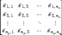
A sequence of N transfer functions in the tf format described above, where N 1. These are assumed to be the individual elements of a transfer-function matrix:

Thus it should be clear that N must be an integer multiple (nu) of the number of outputs, ny.

Also, tfd2mod assumes that you are supplying the transfer functions in a column-wise order. In other words, you should first give the ny transfer functions for input 1 (g_1,1 to gny, 1), then the ny transfer functions for input 2 (g_1,2 to gny, 2), etc.

tfd2mod converts the transfer functions to discrete-time, if necessary, and combines them to form the output variable, model, which is a composite system in the MPC mod form.

Example
Consider the linear system:

The following commands build separate models of the response to the manipulated variables, u, and the unmeasured disturbance, w, all for a sampling period T = 3 then combines them using addumd to get a model of the entire system (the pmod variable):

g11=poly2tfd(12.8,[16.7 1],0,1);
g21=poly2tfd(6.6,[10.9 1],0,7);
g12=poly2tfd(-18.9,[21.0 1],0,3);
g22=poly2tfd(-19.4,[14.4 1],0,3);
delt=3; ny=2;
umod=tfd2mod(delt,ny,g11,g21,g12,g22);
gw1=poly2tfd(3.8,[14.9 1],0,8);
gw2=poly2tfd(4.9,[13.2 1],0,3);
wmod=tfd2mod(delt,ny,gw1,gw2);
pmod=addumd(umod,wmod);

Restriction
The current limit on the number of input transfer functions is N = 25.

See Also
mod, poly2tfd, tfd2step

svdfrsp tfd2step