mod2ss (Model Predictive Control Toolbox)

Model Predictive Control Toolbox

mod2ss

Extracts the standard discrete-time state-space matrices and other information from a model stored in the MPC mod format.

Syntax

[phi,gam,c,d] = mod2ss(mod) 
[phi,gam,c,d,minfo] = mod2ss(mod)

Description

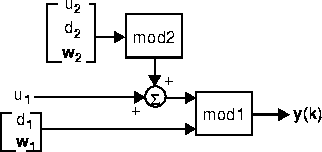
Consider the process shown in the above block diagram. mod2ss assumes that mod is a description of the above process in the MPC mod format (see mod in the online MATLAB Function Reference for more details). An equivalent state-space representation is:

where x is a vector of n state variables, u represents the nu manipulated variables, d represents nd measured but freely-varying inputs (i.e., measured disturbances), w represents nw unmeasured disturbances, y is a vector of ny plant outputs, z is measurement noise, and , u, etc., are constant matrices of appropriate size. The variable (k) represents the plant output before the addition of measurement noise. Define:

= [u d w]

D = [Du Dd Dw]

mod2ss extracts the , , C, and D matrices from the input variable, mod. It also extracts the vector minfo, which contains additional information about the sampling period, number of each type of input and output, etc. see mod in the online MATLAB Function Reference for more details on minfo.

Examples

1.: See the example in the description of dlqe2.

2.: Suppose you have a plant with the structure

where the inputs and outputs are all scalars, and you have constructed mod1 and mod2 using the commands:

phi1=diag([-0.7, 0.8]); gam1=[1, -1, 0; 0, 0, 1]; 
c1=[0.2 -0.4]; d1=zeros(1,3); 
minfo1=[1 2 1 1 1 1 0]; 
mod1=ss2mod(phi1,gam1,c1,d1,minfo1);
phi2=-0.2; gam2=[1, -0.5, 0.2]; 
c2=3; d2=[0.2, 0, 0]; 
minfo2=[1 1 1 1 1 1 0]; 
mod2=ss2mod(phi2,gam2,c2,d2,minfo2); 
pmod=addmod(mod1,mod2);

Now you want to calculate the response to a step change in d₂, which is the fourth input to the composite system, pmod. One way to do it is:

[phi,gam,c,d,minfo]=mod2ss(pmod); 
nstep=10; 
ustep=[zeros(nstep,3) ones(nstep,1) zeros(nstep,2)]; 
% Define step in d2 
y=dlsimm(phi,gam,c,d,ustep); 
% simulate response to step input 
plot([0:nstep-1],y)

The results of the mod2ss call are:

phi=
-0.7000         0     3.0000
      0    0.8000          0
      0         0    -2.0000

gam= 
1.0000     2.2000    -1.0000       0         0         0
                0
     0          0          0       0    1.0000         0 
     0     1.0000          0  -.5000         0    0.2000
c=
0.2000    -0.4000          0 
d=
     0          0          0       0         0         0
minfo=
     1          3          2       2         2         1        0

And the step response is:

See Also
mod, ss2mod

mod2mod mod2step, step format