Mapping Toolbox

Projection Computations

Most of the examples in this document assume that the end product of a map projection is a graphical representation of the map. While this is true for most cases, there may be times when you need access to the non-geographic coordinates of your map data in the projected space.

An easy way to retrieve the projected coordinates of a map that has already been displayed is with the MATLAB get command. The projected coordinates are stored in the object's XData and YData properties. As an example, display a map frame for the Mollweide projection, and extract its x-y coordinates:

• axesm mollweid
  h = framem;
  x = get(h,'XData');
  y = get(h,'YData');
  

Of course, you do not need to display a map object to get its projected coordinates. You can perform the same projection computations that are done within the Mapping Toolbox display commands.

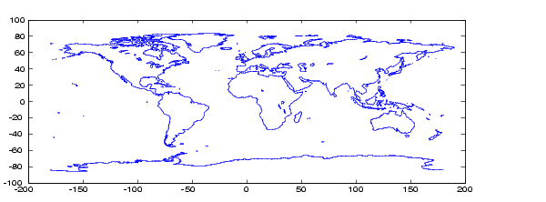
Begin by displaying a map of the coast vector data:

• figure
  load coast
  plot(long,lat); axis equal
  set(gca,'XLim',[-200 200],'YLim',[-100 100])
  

Here is the result. Note that some of the data extends beyond 180° longitude.

Before projecting the data, you must define the projection parameters, just as you would prepare a map axes with axesm before displaying a map. The projection parameters are stored in a map projection structure that normally resides in the UserData property of a MATLAB axes, but you can use it directly for the projection computation.

The following commands create an empty map projection structure for a Sinusoidal projection, change the map origin, and fill in the rest of the structure fields with default property values. Just as you can change the property settings of a map axes with setm, you can use the entries of the map projection structure to control the projection properties.

• mstruct = defaultm('sinusoid');
  mstruct.origin = [0 180 0];
  mstruct = defaultm(sinusoid(mstruct));
  

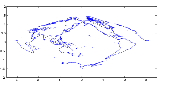
Having defined the map projection parameters, you can project the latitude and longitude vectors into the proper coordinates of the Sinusoidal projection and display the result using non-mapping, MATLAB commands.

• [x,y] = mfwdtran(mstruct,lat,long,[],'line');
  plot(x,y); axis equal
  set(gca,'XLim',[-3.5 3.5],'YLim',[-2 2])
  
  
  
  
  
  
  

For the transformation function, an empty matrix is used to take the place of altitude data, and the string 'line' identifies the object type and allows the vector data to be clipped and trimmed. Notice that the International Date Line is now at the center of the map (180°), as specified earlier.

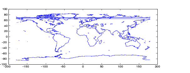
You can transform the projected x-y data back into the Greenwich geographic coordinates with the inverse transformation function. Plot the result:

• [lat2,long2] = minvtran(mstruct,x,y);
  plot(long2,lat2); axis equal
  set(gca,'XLim',[-200 200],'YLim',[-100 100])
  
  
  

What happened? Recall that the original data extended beyond 180° longitude. In the projection transformation process, longitude data outside [-180 180] degrees is projected back into this range since angles differing by 360° are geographically equivalent. The data from the inverse transformation process therefore jumps from 180° to -180°, as depicted by the straight horizontal lines in the figure above. The smoothlong function can be used to remove discontinuities in longitude.

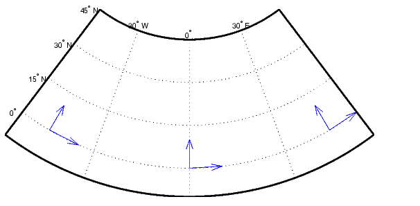
In addition to projecting geographic positions into Cartesian coordinates, you can project angles between the sphere and the plane. For cylindrical projections, north maps to up on the y-axis, and east maps to right on the x-axis. This is not necessarily true of other projections. In conic projections, for example, north may be to the left or right of the y-axis, depending on the geographic coordinates.

What are the angles of north and east in projected coordinates for an equidistant conic? Geographic angles are measured clockwise from north, while projected angles are measured counterclockwise from the x-axis.

• vfwdtran([0 0 0],[-45 0 45],[0 0 0])
  ans =
         59.614           90       120.39
  
  vfwdtran([0 0 0],[-45 0 45],[90 90 90])
  ans =
        -30.385    0.0001931       30.386
  

Coordinate Transformations

Working with the Globe Projection