| Mapping Toolbox | |
Advanced Very High Resolution Radiometer (AVHRR) Global Change Data
The National Oceanic and Atmospheric Administration (NOAA) and others have compiled a global high resolution set of land vegetation measurements to monitor global climate change. The data is derived from the Advanced Very High Resolution Radiometer (AVHRR) sensor carried on NOAA meteorological satellites (NOAA-7, -9, 11). The sensor measures reflected radiation in five different wave-bands with a 1 km spatial resolution, which is then processed into a Non-dimensional Vegetation Index (NDVI). The NDVI has been used as the basis for a global landcover classification dataset. Other applications of the AVHRR data include oceanographic and atmospheric science. Many of those datasets are stored in HDF formats, which can be read using the MATLAB imread or hdfread functions. This section focuses on the land datasets, which are stored in several different map projections and require special interface functions.
Low resolution monthly NDVI composites are available from
<ftp://daac.gsfc.nasa.gov/data/inter_disc/biosphere/avhrr_ndvi/>
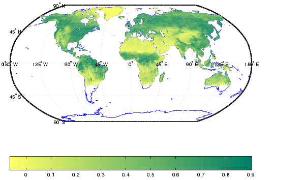
These are binary files stored as a 1 degree geographic grid. You can read these files with readmtx, a Mapping Toolbox function that reads matrices stored in files based on a description of the file format. Here is an example of the non-dimensional vegetation index data for September 1994. This data was retrieved from <ftp://daac.gsfc.nasa.gov/data/inter_disc/biosphere/avhrr_ndvi/1994/avhrr_pf.ndvi.1nmegl.9409.bin>.
map = readmtx('avhrr_pf.ndvi.1nmegl.9409.bin',180,360,'real*4');
map = flipud(map);
map(map<-9)=NaN;
maplegend = [1 90 -180];
worldmap('world','none'); plotm(coast);
meshm(map,maplegend,size(map))
colormap(flipud(summer))
colorbar('horiz')
What are the values of the non-dimensional vegetation index at particular locations?
[lat,lon] = extractm(worldlo('gazette'),...
     {'Vancouver','Oslo','Cairo','Lagos','Tripoli'});
lat = lat(~isnan(lat)); lon = lon(~isnan(lon));
val = ltln2val(map,maplegend,lat,lon);
Other AVHRR products are stored as matrices in projected coordinates. The standard projection for the 1 kilometer resolution data is the interrupted Goode, which can be read using the avhrrgoode interface function. Some of the data is also available in the Lambert Equal-Area Azimuthal projection. Extracting data from the Lambert files with avhrrlambert is much faster. If you have a choice, you should probably read data in the Lambert format.
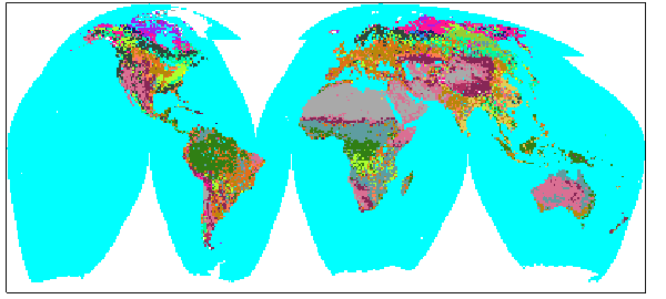
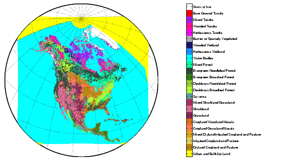
The global 1 kilometers data in the Goode projection is stored as a binary matrix with 17347 rows and 40031 columns. The uncompressed file size is about 695 megabytes, slightly more than the capacity of one CD-ROM disk. Here is an image of the data as it is stored. This example uses the Global Land Cover Classification data in the USGS classification scheme, available from <ftp://edcftp.cr.usgs.gov/pub/data/glcc/globe/gusgs1_2.img.gz>. The colors correspond to different types of vegetation and land use.
nrows = 17347;   % 16347 for some data on cd-rom
ncols = 40031;   % 40031
mtx = readmtx('gusgs1_2.img',nrows,ncols,'int8',...
              1:100:nrows,1:100:ncols);

h = image(mtx);
axis image

load usgslulegend
colormap(cmap); set(h,'CdataMapping','Direct')
showaxes off
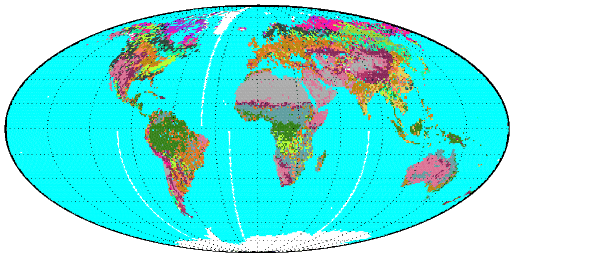
To display this data on a map projection, extract the data with the avhrrgoode function. The next example reads the data at the same resolution as above, returning a general matrix map consisting of the latitude, longitude, and data matrices.
[latgrat,longrat,map] = avhrrgoode('global','gusgs1_2.img',100);
figure; axesm mollweid; framem; gridm;
surfm(latgrat,longrat,map); colormap(cmap)
set(handlem('surface'),'CdataMapping','Direct')
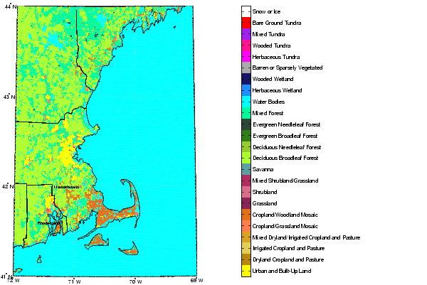
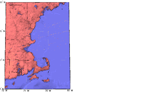
You can read the data for just a part of the world and control the resolution of the extracted data and the size of the graticule matrices. Data is sometimes provided in regional subsets of the very large global Goode files. You can read these by supplying the name of the region. For example, read the USGS land cover data for Cape Cod at the full resolution from the North America file, available from <ftp://edcftp.cr.usgs.gov/pub/data/glcc/na/goode/nausgs1_2g.img.gz>.
latlim = [41 44]; lonlim = [-72 -69];
[latgrat,longrat,map] = avhrrgoode('north america',...
     'nausgs1_2g.img',1,latlim,lonlim);
usamap(latlim,lonlim,'line')
surfm(latgrat,longrat,map); colormap(cmap)
set(handlem('surface'),'CDataMapping','Direct')
set(gca,'Position',[.1 .1 .5 .8])
caxis([.5 24.5]); hcb = colorbar;
set(hcb,'YTick',1:24,'YTickLabel',USGSLandUse,...
    'Position',[.6 .1 .02 .8])
The full matrix of AVHRR data is too large to fit on one CD-ROM disk. When the data is provided on CD-ROM, the size of the data is reduced by dropping the last rows. To read the truncated files, specify the number of rows and columns in the non-standard file. This information can usually be found in the `Readme' file. Here is the non-dimensional vegetation index data for Cape Cod from the "Global Land 1-km AVHRR Data Set - Vegetation Index 6/21-30, 1992" CD-ROM (distributed by the Land Processes Distributed Active Archive Center, EROS Data Center, Sioux Falls, South Dakota, 57198, USA). The empty matrix argument specifies that the graticule size will be the same size as the map. The geographic registration for this older CD seems to be less accurate.
[latgrat,longrat,map] = avhrrgoode('global','NDVI.IMG',...
     1,latlim,lonlim,[],16347,40031);
figure
usamap(latlim,lonlim,'line')
surfm(latgrat,longrat,map)
% Lighten the colormap
cmap = flipud(jet(64));
hsvmap = rgb2hsv(cmap); hsvmap(:,2) = .5; cmap = hsv2rgb(hsvmap);
colormap(cmap)
AVHRR data is also available in the Goode projection at a resolution of 8 kilometers. You can read the global 8 km files with avhrrgoode, but not the 8 km regional files.
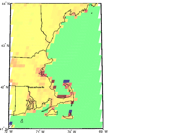
Read the global 8 km resolution non-dimensional vegetation index for Cape Cod. This data file is available from
<ftp://daac.gsfc.nasa.gov/data/avhrr/global_8km/.1994_1997/1994/jun/avhrrpf.ndvi.1ntfgl.940621.gz>
Specify the non-standard number of rows, columns, and resolution in the file. The jagged edges in the surface are a result of trimming a slanted graticule to the map frame.
[latgrat,longrat,map] = avhrrgoode('global',...
     'avhrrpf.ndvi.1ntfgl.940621',1,...
     latlim,lonlim,[],2168,5004,8000);
clmo surface
surfm(latgrat,longrat,map)
Regional versions of the 1 km Global Land Cover Classification data are also available saved in Lambert azimuthal equal area projections. These can be read using the avhrrlambert function. Reading data from the Lambert projection will be faster than from the interrupted Goode, because the graticule does not need to be trimmed to the boundaries of the individual projection zones.
Read the Global Land Cover Characteristics (GLCC) file covering North America in the Lambert projection with the USGS classification scheme. This file is available from <ftp://edcftp.cr.usgs.gov/pub/data/glcc/na/lambert/nausgs1_2l.img.gz>.
[latgrat,longrat,map] = avhrrlambert('north america',...
                                     'nausgs1_2l.img',25);

axesm('eqdazim','Origin',[50 -100],'FLatLimit',[-Inf 50],...
      'mlinelocation',15); framem; gridm
surfm(latgrat,longrat,map)
load usgslulegend; colormap(cmap)
set(handlem('surface'),'CDataMapping','Direct'); tightmap
caxis([.5 24.5]); hcb = colorbar;
set(hcb,'YTick',1:24,'YTickLabel',USGSLandUse,...
    'Position',[.7 .1 .02 .8])
set(gca,'Position',[-.05 .1 .8 .8])
It is sometimes useful to drape land cover data onto elevation maps. The elevation data is displayed as a three-dimensional surface, onto which the new land cover map is texture mapped. The lighting effects allow you to see the land use change from intensive agriculture in low-lying flatlands to mixed cropland and woodland, and finally to pure woodland in more mountainous areas. Here are two examples combining the Global Land Cover Classification data with the GTOPO30 elevations. The first converts the general matrix map of land cover codes to a regular matrix map and combines it with a regular matrix map of elevations.
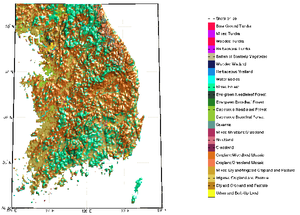
latlim = [34 38.5]; lonlim = [126 130];
% <ftp://edcftp.cr.usgs.gov/pub/data/glcc/ea/lamberta/
%        eausgs1_2la.img.gz>
[latgrat,longrat,mat] = avhrrlambert('asia',...
     'eausgs1_2la.img',1,latlim,lonlim);
[lcmap,lcmaplegend] = nanm(latlim,lonlim,.7/km2deg(1));
lcmap = imbedm(latgrat,longrat,mat,lcmap,lcmaplegend);
% <ftp://edcftp.cr.usgs.gov/pub/data/gtopo30/global/
%        e100n40.tar.gz>
[map,maplegend] = gtopo30('e100n40',2,latlim,lonlim);
worldmap(latlim,lonlim,'none')
h = meshm(map,maplegend,size(map),map)
set(h,'FaceColor','texturemap','CData',lcmap)
colormap(cmap)  % predefined colormap
set(h,'CDataMapping','direct')  % integer land cover codes
set(gca,'Position',[.1 .1 .5 .8])
daspectm('m',10); camlight; lighting phong;
caxis([.5 24.5]); hcb = colorbar;
set(hcb,'YTick',1:24,'YTickLabel',USGSLandUse,...
     'Position',[.6 .1 .02 .8])
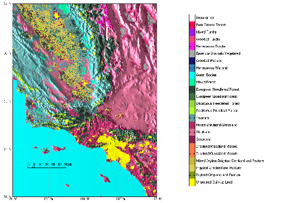
The other approach is to interpolate a regular matrix map of elevations into a the general matrix. Here is an example using the land cover data and elevations for Southern California. You can see how forests are predominantly at the higher elevations around Los Angeles and the San Joaquin Valley. Notice also the string of urban areas along the treeline of the Sierra Nevada Mountains. These do not appear in other map sources, and may be spurious.
latlim = [33 37]; lonlim = [-121 -117]; % socal
[latgrat,longrat,lcmap] = avhrrlambert('north america',...
     'nausgs1_2l.img',1,latlim,lonlim);
latgratlim = [min(latgrat(:)) max(latgrat(:))];
longratlim = [min(longrat(:)) max(longrat(:))];
[elmap,elmaplegend] = gtopo30('W140N40',1,...
     latgratlim,longratlim);
elmap(isnan(elmap)) = -1;
z = ltln2val(elmap,elmaplegend,latgrat,longrat);
figure; worldmap(latlim,lonlim,'none');
setm(gca,'MapProjection','mercator')
hs = surfm(latgrat,longrat,lcmap,z);
set(hs,'CDataMapping','direct')
load usgslulegend; colormap(cmap)
daspectm('m',5); material([0.6 2 0])
camlight(-80,0); lighting phong
caxis([.5 24.5]); hcb = colorbar;
set(hcb,'YTick',1:24,'YTickLabel',USGSLandUse,...
     'Position',[.7 .1 .02 .8])
set(gca,'Position',[-0.04.05 .8 .9])
scaleruler('Units','mi'); tightmap
| | Reading Elevation Data Interactively | EGM96 Geoid Model | |