predint (Curve Fitting Toolbox)

Compute prediction bounds for new observations or for the function

Syntax

ci = predint(fresult,x)
ci = predint(fresult,x,level)
ci = predint(fresult,x,level,'intopt','simopt')
[ci,ypred] = predint(...)

Arguments

fresult
A fit result object.

x
The values at which predictions are calculated.

level
Confidence level. The value must be between 0 and 1. The default value is 0.95.

'intopt'
Can be observation (the default) to compute bounds for new response values, or functional to compute bounds for the fit evaluated at x.

'simopt'
Can be off (the default) to compute nonsimultaneous bounds, or on to compute simultaneous bounds.

ci
An array of upper and lower prediction bounds.

ypred
The predicted (fitted) value of fresult evaluated at x.

`fresult`	A fit result object.
`x`	The values at which predictions are calculated.
`level`	Confidence level. The value must be between 0 and 1. The default value is 0.95.
`'intopt'`	Can be `observation` (the default) to compute bounds for new response values, or `functional` to compute bounds for the fit evaluated at `x`.
`'simopt'`	Can be `off` (the default) to compute nonsimultaneous bounds, or `on` to compute simultaneous bounds.
`ci`	An array of upper and lower prediction bounds.
`ypred`	The predicted (fitted) value of `fresult` evaluated at `x`.

Description

ci = predint(fresult,x) returns prediction bounds for new response (observation) values at the predictor values specified by x. The confidence level of the predictions is 95%. ci contains the upper and lower prediction bounds. fresult is the fit result object returned by the fit function. You can compute prediction bounds only for parametric fits. To compute confidence bounds for the fitted parameters, use the confint function.

ci = predint(fresult,x,level) returns prediction bounds with a confidence level specified by level.

ci = predint(fitresult,x,level,'intopt','simopt') specifies the type of bounds to compute. If intopt is functional, the bounds measure the uncertainty in estimating the function (the fitted curve). If intopt is observation, the bounds are wider to represent the additional uncertainty in predicting a new response value (the fitted curve plus random noise).

If simopt is off, nonsimultaneous bounds are calculated. If simopt is on, simultaneous bounds are calculated. Nonsimultaneous bounds take into account only individual x values. Simultaneous bounds take into account all x values.

[ci,ypred] = predint(...) returns the predicted (fitted) value of fresult evaluated at x.

Example

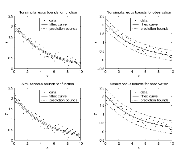
Generate some data and add noise.

x = (0:0.2:10)';
coef = [2 -0.2];
rand('state',0)
y = coef(1)*exp(coef(2)*x) + (rand(size(x))-0.5)*0.5;

Fit the data using a single-term exponential and define the range over which prediction bounds are calculated.

```
fresult = fit(x,y,'exp1');
```

Return the prediction bounds for the function as well as the predicted values of the fit using nonsimultaneous and simultaneous bounds with a 95% confidence level. For nonsimultaneous bounds, given a single predetermined predictor value, you have 95% confidence that the true function lies between the confidence bounds. For simultaneous bounds, you have 95% confidence that the function at all predictor values lies between the bounds.

[c1,ypred1] = predint(fresult,x,0.95,'fun','off');
[c2,ypred2] = predint(fresult,x,0.95,'fun','on');

Return the prediction bounds for new observations as well as the predicted values of the fit using nonsimultaneous and simultaneous bounds with a 95% confidence level. For nonsimultaneous bounds, given a single predictor value, you have 95% confidence that a new observation lies between the confidence bounds. For simultaneous bounds, regardless of the predictor value, you have 95% confidence that a new observation lies between the bounds.

[c3,ypred3] = predint(fresult,x,0.95,'obs','off');
[c4,ypred4] = predint(fresult,x,0.95,'obs','on');

Plot the data, fit, and confidence bounds.

subplot(2,2,1), plot(fresult,x,y), hold on, plot(x,c1,'k-.')
legend('data','fitted curve','prediction bounds')
title('Nonsimultaneous bounds for function')
subplot(2,2,3), plot(fresult,x,y), hold on, plot(x,c2,'k-.')
legend('data','fitted curve','prediction bounds')
title('Simultaneous bounds for function')
subplot(2,2,2), plot(fresult,x,y), hold on; plot(x,c3,'k-.')
legend('data','fitted curve','prediction bounds')
title('Nonsimultaneous bounds for observation')
subplot(2,2,4), plot(fresult,x,y), hold on, plot(x,c4,'k-.')
legend('data','fitted curve','prediction bounds')
title('Simultaneous bounds for observation')

See Also

confint, fit

plot set