SimPowerSystems

Phasor Simulation of a Circuit Transient

You now apply the phasor solution method to a simple linear circuit. Open the Demos library of powerlib. Open the Simple Demos library and select the demo named "Transient Analysis". A system named psbtransient opens.

Figure 1-16: Simple Linear Circuit Built in Power System Blockset

This circuit is a simplified model of a 60 Hz, 230 kV three-phase power system where only one phase is represented. The equivalent source is modeled by a voltage source (230 kV rms / sqrt(3) or 132.8 kV rms, 60 Hz) in series with its internal impedance (Rs Ls). The source feeds a RL load through a 150 km transmission line modeled by a single PI section (RL1 branch and two shunt capacitances, C1 and C2). A circuit breaker is used to switch the load (75 MW, 20 Mvar) at the receiving end of the transmission line. Two measurement blocks are used to monitor the load voltage and current.

The Powergui block at the lower right corner indicates that the model is continuous. Start the simulation and observe transients in voltage and current waveforms when the load is first switched off at t = 0.0333 s (2 cycles) and switched on again at t = 0.1167 s (7 cycles).

Invoking the Phasor Solution in the Powergui Block

You now simulate the same circuit using the phasor simulation method. This option is accessible through the Powergui block. Open this block and select Phasor simulation. You must also specify the frequency used to solve the algebraic network equations. A default value of 60 Hz should already be entered in the Frequency menu. Close the Powergui and notice that the word Phasors now appears on the Powergui icon, indicating that the Powergui now applies this method to simulate your circuit.

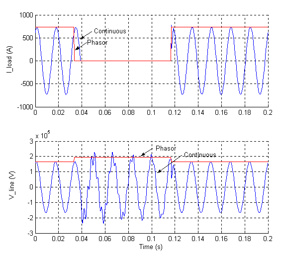
Restart the simulation. The magnitudes of the 60 Hz voltage and current are now displayed on the scope. Waveforms obtained from the continuous simulation and the phasor simulation are superimposed in this plot.

Figure 1-17: Waveforms Obtained with the Continuous and Phasor Simulation Methods

Note that with continuous simulation, the opening of circuit breaker occurs at the next zero crossing of current following the opening order; whereas for the phasor simulation, this opening is instantaneous. This is because there is no concept of zero crossing in the phasor simulation.

Selecting Phasor Signal Measurement Formats

If you now double-click the voltage measurement block or the current measurement block, you see that a menu allows you to output phasor signals in four different formats: Complex, Real-Imag, Magnitude-Angle, or just Magnitude (default choice). If you select Magnitude-Angle, both magnitude and angle (in degrees) are multiplexed at the output of the measurement block. You might need to demultiplex these two signals to send them on separate traces of the scope. Note that the oscilloscope does not accept complex signals. You should instead use the Real-Imag format.

The Complex format allows the use of complex operations and processing of phasors without separating real and imaginary parts. Suppose for example that you need to compute the power consumption of the load (active power P and reactive power Q). The complex power S is obtained from the voltage and current phasors as

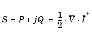
where I* is the conjugate of the current phasor. The 1/2 factor is required to convert magnitudes of voltage and current from peak values to rms values.

Select the Complex format for both current and voltage and, using blocks from the Simulink Math library, implement the power measurement as shown.

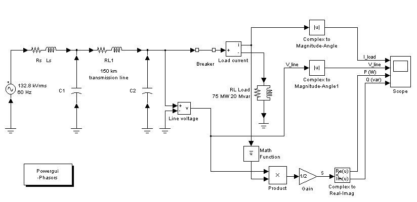
Figure 1-18: Power Computation Using Complex Voltage and Current

The Complex to Magnitude blocks are now required to convert complex phasors to magnitudes before sending them to the scope.

The power computation system you just implemented is already built in the Power System Blockset: the Active and Reactive Power (Phasor Type) block is available in the Extras library under the Phasor collection of blocks.

Session 6: Introducing the Phasor Simulation Method

Session 7: Three-Phase Systems and Machines