SimMechanics

Linearizing SimMechanics Models

The Simulink linmod command creates linear time-invariant (LTI) state-space models from Simulink models. You can use this command to generate an LTI state-space model from a SimMechanics model, for example, to serve as input to Control System Toolbox commands that generate controller models. The linmod command allows you to specify the point in state space about which it linearizes the model (the operating point). You should choose a point where your model is in equilibrium, i.e., where the net force on the model is zero. You can use the Simulink trim command to find a suitable operating point (see Trimming Mechanical Systems). By default linmod uses an adaptive perturbation method to linearize a SimMechanics model. The Mechanical Environment Settings dialog box allows you to specify that linmod use a fixed perturbation method instead (see Linearization Pane). The following example illustrates the use of linmod to linearize a SimMechanics model.

Note    Before linearizing a model, perform at least one simulation in Forward Dynamics mode. See Choosing an Analysis Mode.

Model Linearization Example: Double Pendulum

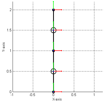
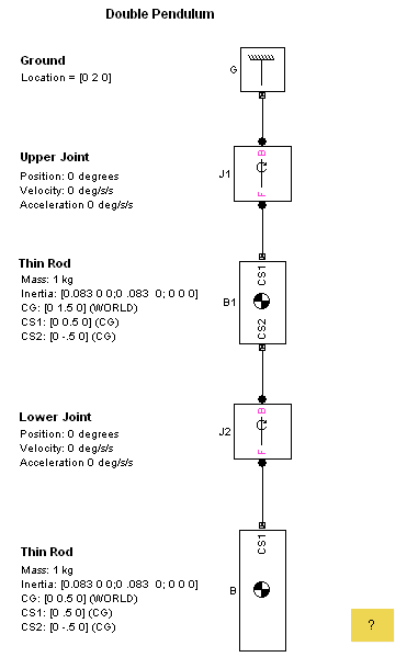
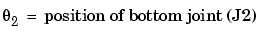
Consider a double pendulum initially hanging straight up and down.

The net force on the pendulum is zero in this configuration. The pendulum is thus in equilibrium.

The following figure shows a SimMechanics demo model of the pendulum, mech_dpend_forw.

To linearize this model, enter

• [A B C D] = linmod('mech_dpend_forw');
  

at the MATLAB command line. This form of the linmod command linearizes the model about the model's initial states.

Note    The linmod command ignores initial states specified by Initial Condition blocks. If you want to linearize a model about an operating point partly or entirely specified by IC blocks, you must pass an initial state vector to the linmod command. Similarly, if the system to be linearized has inputs, you must pass an initial input vector to the linmod command. See the Simulink documentation on the linmod command for more information. The double pendulum model in this example contains no IC blocks or inputs. It is therefore unnecessary to pass any additional arguments (other than the model's name) to the command to linearize the model.

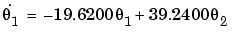
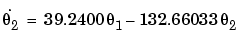
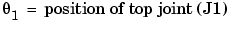
The matrices A, B, C, D returned by the linmod command correspond to the standard mathematical representation of an LTI state-space model:

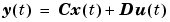
where x is the model's state vector, y is its outputs, and u is its inputs. The double pendulum model has no inputs or outputs. Consequently, only A is not null. This reduces the state-space model for the double pendulum to

where

• A =
  
           0         0    1.0000         0
           0         0         0    1.0000
   -137.3400   39.2400         0         0
     39.2400  -19.6200         0         0
  
  

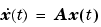
This model specifies the relationship between the state derivatives and the states of the double pendulum. The state vector of the LTI model has the same format as the state vector of the SimMechanics model. The SimMechanics mech_stateVectorMgr command gives the format of the state vector as follows:

• vm = mech_stateVectorMgr('mech_dpend_forw/G');
  
  ans = 
  
      'mech_dpend_forw/J2:R1:Position'
      'mech_dpend_forw/J1:R1:Position'
      'mech_dpend_forw/J2:R1:Velocity'
      'mech_dpend_forw/J1:R1:Velocity'
  

Multiplying A by the state vector x yields the differential state equations corresponding to the LTI model of the double pendulum.

where

The following Simulink model implements the state space model represented by these equations.

This model in turn allows creation of a model, located in mech_dpend_lin, that computes the LTI approximation error.

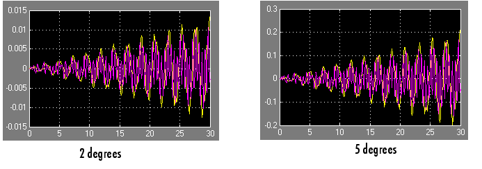
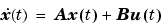
Running the model twice with the upper joint deflected 2 degrees and 5 degrees, respectively, shows an increase in error as the initial state of the system strays from the pendulum's equilibrium position and as time elapses. This is the expected behavior of a linear state-space approximation.

Constrained Example: Four-Bar System

How SimMechanics Works