Partial Differential Equation Toolbox

hyperbolic

Solve hyperbolic PDE problem

Syntax

• u1=hyperbolic(u0,ut0,tlist,b,p,e,t,c,a,f,d) 
  u1=hyperbolic(u0,ut0,tlist,b,p,e,t,c,a,f,d,rtol) 
  u1=hyperbolic(u0,ut0,tlist,b,p,e,t,c,a,f,d,rtol,atol) 
  u1=hyperbolic(u0,ut0,tlist,K,F,B,ud,M) 
  u1=hyperbolic(u0,ut0,tlist,K,F,B,ud,M,rtol) 
  u1=hyperbolic(u0,ut0,tlist,K,F,B,ud,M,rtol,atol)
  

Description

u1=hyperbolic(u0,ut0,tlist,b,p,e,t,c,a,f,d) produces the solution to the FEM formulation of the scalar PDE problem

or the system PDE problem

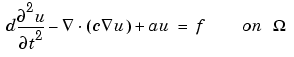
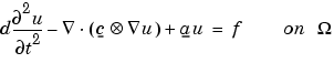
on a mesh described by p, e, and t, with boundary conditions given by b, and with initial value u0 and initial derivative ut0.

In the scalar case, each row in the solution matrix u1 is the solution at the coordinates given by the corresponding column in p. Each column in u1 is the solution at the time given by the corresponding item in tlist. For a system of dimension N with np node points, the first np rows of u1 describe the first component of u, the following np rows of u1 describe the second component of u, and so on. Thus, the components of u are placed in blocks u as N blocks of node point rows.

b describes the boundary conditions of the PDE problem. b can be either a Boundary Condition matrix or the name of a Boundary M-file. The boundary conditions can depend on t, the time. The formats of the Boundary Condition matrix and Boundary M-file are described in the entries on assemb and pdebound, respectively.

The geometry of the PDE problem is given by the mesh data p, e, and t. For details on the mesh data representation, see initmesh.

The coefficients c, a, d, and f of the PDE problem can be given in a variety of ways. The coefficients can depend on t, the time. For a complete listing of all options, see assempde.

atol and rtol are absolute and relative tolerances that are passed to the ODE solver.

u1=hyperbolic(u0,ut0,tlist,K,F,B,ud,M) produces the solution to the ODE problem

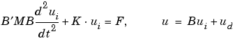
with initial values for u being u0 and ut0.

Examples

Solve the wave equation

on a square geometry -1 x,y 1 (squareg), with Dirichlet boundary conditions u = 0 for x = ±1, and Neumann boundary conditions

for y = ±1 (squareb3). Choose

and

Compute the solution at times 0, 1/6, 1/3, ... , 29/6, 5.

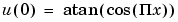
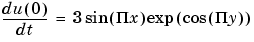
• [p,e,t]=initmesh('squareg'); 
  x=p(1,:)'; 
  y=p(2,:)'; 
  u0=atan(cos(pi/2*x)); 
  ut0=3*sin(pi*x).*exp(cos(pi*y)); 
  tlist=linspace(0,5,31); 
  uu=hyperbolic(u0,ut0,tlist,'squareb3',p,e,t,1,0,0,1); 
  

The file pdedemo6 contains a complete example with animation.

Note    In expressions for boundary conditions and PDE coefficients, the symbol t is used to denote time. The variable t is often used to store the triangle matrix of the mesh. You can use any variable to store the triangle matrix, but in PDE toolbox expressions, t always denotes time.

See Also

assempde, parabolic

dst, idst

initmesh