
| Partial Differential Equation Toolbox |   |
Structural Mechanics -- Plane Stress
In structural mechanics, the equations relating stress and strain arise from the balance of forces in the material medium. Plane stress is a condition that prevails in a flat plate in the xy plane, loaded only in its own plane and without z-direction restraint.
The stress-strain relation can then be written, assuming isotropic and isothermal conditions

where  x and
x and  y are the stresses in the x and y directions, and
  xy is the shear stress. The material properties are expressed as a combination of E, the elastic modulus or Young's modulus, and
  , Poisson's ratio.
The deformation of the material is described by the displacements in the x and y directions, u and v, from which the strains are defined as

The balance of force equations are

where Kx and Ky are volume forces (body forces).
Combining the relations above, we arrive at the displacement equations, which can be written
 · (c
· (c 
 u) = k
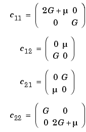
where c is a rank four tensor, which can be written as four 2-by-2 matrices
c11, c12, c21, and c22:

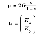
where G, the shear modulus, is defined by


This is an elliptic PDE of system type (u is two-dimensional), but you need only to select the application mode Structural Mechanics, Plane Stress and then enter the material-dependent parameters E and  and the volume forces k into the PDE Specification dialog box.
In this mode, you can also solve the eigenvalue problem, which is described by
 · (c
· (c 
 u) =
u) =  du
du

 , the density, can also be entered using the PDE Specification dialog box.
In the Plot Selection dialog box, the x- and y-displacements, u and v, and the absolute value of the displacement vector (u,v) can be visualized using color, contour lines, or z-height, and the displacement vector field (u,v) can be plotted using arrows or a deformed mesh. In addition, for visualization using color, contour lines, or height, you can choose from 15 scalar tensor expressions:


exx, the x-direction strain ( x)
x)
eyy, the y-direction strain ( y)
y)
exy, the shear strain ( xy)
xy)
sxx, the x-direction stress ( x)
x)
syy, the y-direction stress ( y)
y)
sxy, the shear stress ( xy)
xy)
e1, the first principal strain ( 1)
1)
e2, the second principal strain ( 2)
2)
s1, the first principal stress ( 1)
1)
s2, the second principal stress ( 2)
2)
von Mises, the von Mises effective stress

For a more detailed discussion on the theory of stress-strain relations and applications of FEM to problems in structural mechanics, see [1].
Example
Consider a steel plate that is clamped along a right-angle inset at the lower left corner, and pulled along a rounded cut at the upper right corner. All other sides are free.
The steel plate has the following properties: Dimension: 1-by-1 meters; thickness 1mm; inset is 1/3-by-1/3 meters. The rounded cut runs from (2/3, 1) to (1, 2/3). Young's modulus: 196 · 103 (MN/m2), Poisson's ratio: 0.31.
The curved boundary is subjected to an outward normal load of 500 N/m. We need to specify a surface traction; we therefore divide by the thickness 1 mm, thus the surface tractions should be set to 0.5 MN/m2. We will use the force unit MN in this example.
We want to compute a number of interesting quantities, such as the x- and y-direction strains and stresses, the shear stress, and the von Mises effective stress.
Using the Graphical User Interface
Using the pdetool GUI, the first thing to do is to select the application mode. For this problem, use Structural Mechanics, Plane Stress.
The CSG model can be made very quickly by drawing a polygon with corners in x=[0 2/3 1 1 1/3 1/3 0] and y=[1 1 2/3 0 0 1/3 1/3] and a circle with center in x=2/3, y=2/3 and radius 1/3.
The polygon is normally labeled P1 and the circle C1, and the CSG model of the steel plate is simply P1+C1.
Next, select Boundary Mode to specify the boundary conditions. First, remove all subdomain borders by selecting Remove All Subdomain Borders . . . from the Boundary menu. The two boundaries at the inset in the lower left are clamped, i.e., Dirichlet conditions with zero displacements. The rounded cut is subject to a Neumann condition with q=0 and g1=0.5*nx, g2=0.5*ny. The remaining boundaries are free (no normal stress), that is, a Neumann condition with q=0 and g=0.
The next step is to open the PDE Specification dialog box and enter the PDE parameters.
The E and  (
(nu) parameters are Young's modulus and Poisson's ratio, respectively. There are no volume forces, so Kx and Ky are zero.  (
(rho) is not used in this mode. The material is homogeneous, so the same E and  apply to the whole 2-D domain.
Initialize the mesh by clicking the  button. If you want, you can refine the mesh by clicking the Refine button.
The problem can now be solved by clicking the = button.
A number of different strain and stress properties can be visualized, such as the displacements u and v, the x- and y-direction strains and stresses, the shear stress, the von Mises effective stress, and the principal stresses and strains. All these properties can be selected from pop-up menus in the Plot Selection dialog box. A combination of scalar and vector properties can be plotted simultaneously by selecting different properties to be represented by color, height, vector field arrows, and displacements in a 3-D plot.
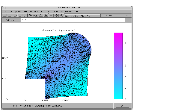
Select to plot the von Mises effective stress using color and the displacement vector field (u,v) using a deformed mesh. Select the Color and Deformed mesh plot types. To plot the von Mises effective stress, select von Mises from the pop-up menu in the Color row.
In areas where the gradient of the solution (the stress) is large, you need to refine the mesh in order to increase the accuracy of the solution. Select Parameters . . . from the Solve menu and check the Adaptive mode option. You can use the default options for adaption, which are the Worst triangles triangle selection method with the Worst triangle fraction set to 0.5. Now solve the plane stress problem again. Select the Show Mesh option in the Plot Selection dialog box to see how the mesh is refined in areas where the stress is large.

Visualization of the von Mises Effective Stress and the Displacements Using Deformed Mesh
 | The Application Modes and the GUI | Structural Mechanics -- Plane Strain |  |